Data Structures and Algorithms
- Understand common data structures and common implementations such as arrays, stacks, queues, linked lists, trees, and hash tables
- Learn important algorithms and logic for sorting and searching and understand how to compare their performance
Introduction
A data structure is a way of organising and storing data within programs.
An algorithm is a method of processing data structures.
In general, programming is all about building data structures and then designing algorithms to run on them, but when people talk about “data structures and algorithms” they normally mean the standard building blocks that you put together into your own programs. So in this course, we will be looking at:
- Various standard data structures:
- Lists
- Stacks
- Queues
- Dictionaries or Maps
- Sets
- A few common algorithms:
- Sorting data into order
- Searching through data for a particular value
Part 1 – Algorithmic complexity
Complexity is a general way of talking about how fast a particular operation will be. This is needed to be able to compare different structures and algorithms.
Consider the following pseudocode:
function countRedFruit(basket):
  var count = 0

  foreach fruit in basket:
    if fruit.colour == red:
      count = count + 1

  return count
The answer to the question How long does this take to execute? will depend on many factors such as the language used and the speed of the computer. However, the main factor is going to be the total number of fruit in the basket: if we pass in a basket of 10 million fruit, it will probably take about a million times longer than 10 fruit.
To describe this, we use ‘Big-O Notation’, which is a way of expressing how long the algorithm will take based on the size of the input. If the size of our input is n, then the example above will take approximately n iterations, so we say that the algorithm is O(n).
When using this notation, constant multiples and ‘smaller’ factors are ignored, so the expression contains only the largest term. For example:
| Big O | Description | Explanation | Example |
|---|---|---|---|
| O(1) | Constant Time | The algorithm will always take about the same time, regardless of input size. The algorithm is always very fast | Finding the first element of a list |
| O(log(n)) | Logarithmic Time | The algorithm will take time according to the logarithm of the input size. The algorithm is efficient at handling large inputs | Binary search |
| O(n) | Linear Time | The algorithm will take time proportional to the input size. The algorithm is about as slow for large inputs as you might expect | Counting the elements of a list |
| O(n²) | Quadratic Time | The algorithm will take time quadratic to the input size. The algorithm is inefficient at handling large inputs | Checking for duplicates by comparing every element to every other element |
There are many other possibilities of course, and it’s only really interesting to compare different complexities when you need to choose a known algorithm with a large amount of data.
If we consider the following algorithm:
function countDistinctColours(basket):
  var count = 0

  for i in 0 to basket.length-1:
    var duplicated = false

    for j in 0 to i-1:
      if basket[i].colour == basket[j].colour:
        duplicated = true

    if not duplicated:
      count = count + 1

  return count
This counts the number of different colours in the basket of fruit. Pass in a basket of 10 fruits where 2 are red, 1 is yellow and 7 are green; it will give the answer 3, and it will do so quite quickly. However, pass in a basket of 10 million fruits and it doesn’t just take a million times longer. It will instead take (nearly) a million million times longer (that is, a trillion times longer). The two nested for-loops mean that the size of the basket suddenly has a hugely more significant effect on execution time.
In this case, for each piece of input, we execute the body of the outer loop, inside which there is another loop, which does between 0 and n iterations (depending on i). This means that the overall cost is n * n/2; because constant factors are ignored when considering the complexity, the overall complexity is O(n²).
Speed vs memory
Above we describe computational complexity, but the same approach can be applied to memory complexity, to answer the question How much space do the data structures require to take up?
The code snippet above has a memory complexity of O(1). That is, it uses a fixed amount of memory – an integer. How big these integers are is not relevant – the important point is that as the size of the input gets bigger, the amount of memory used does not change.
Consider the following alternative implementation of countDistinctColours:
function countDistinctColoursQuickly(basket):
  var collection

  for i in 0 to basket.length-1:
    if not collection.contains(basket[i].colour):
      collection.add(basket[i].colour)

  return collection.size
If it is assumed that there is no constraint on how many different colours may exist (so in a basket of a million fruits, each may have a unique colour) then the collection might end up being as big as our basket. Therefore the memory complexity of this algorithm is O(n).
In general, speed is much more important than memory, but in some contexts, the opposite may be true. This is particularly the case in certain tightly constrained systems; for example, the Apollo Guidance system had to operate within approximately 4KB of memory!
Part 2 – Sorting algorithms
This topic looks at algorithms for sorting data. Any programming language’s base library is likely to provide implementations of sorting algorithms already, but there are several reasons why it’s valuable to understand how to build them from scratch:
- It’s worth understanding the performance and other characteristics of the algorithms available to you. While much of the time “any sort will do”, there are situations where the volumes of data or constraints on resources mean that you need to avoid performance issues.
- Sorting algorithms are a good example of algorithms in general and help get into the mindset of building algorithms. You may never need to implement your own sort algorithm, but you will certainly need to build some algorithms of your own in a software development career.
- It may be necessary for you to implement a bespoke sorting algorithm for yourself. This is normally in specialised cases where there are particular performance requirements or the data structure is not compatible with the standard libraries. This will not be a regular occurrence, but many seasoned programmers will have found a need to do this at some point in their careers.
Selection sort
Selection Sort is one of the simplest sorting algorithms. Assume that there is an array of integers, for example:
4,2,1,3
Start by scanning the entire list (array indexes 0 to n-1) to find the smallest element (1) and then swap it with the first element in the list, resulting in:
1,2,4,3
At this point, you know that the first element is in the correct place in the output, but the rest of the list isn’t in order yet. So the exercise is repeated on the rest of the list (array indexes 1 to n-1) to find the smallest element in that sub-array. In this case, it’s 2 – and it’s already in the right place, so it can be left there (or if you prefer, “swap it with itself”).
Finally indexes 2 to n-1 are checked, to find that 3 is the smallest element. 3 is swapped with the element at index 2, to end up with:
1,2,3,4
Now there is only one element left that has not been explicitly put into order, which must be the largest element and has ended up in the correct place at the end of the list.
- Find the smallest element in the list
- Swap this smallest element with the first element in the list
- The first element is now in the correct order. Repeat the algorithm on the rest of the list
- After working through the entire list, stop
Note that each time through the loop one item is found that can be put into the correct place in the output. If there are 10 elements in the list, the loop must be done 10 times to put all the elements into the correct order.
Selection sort analysis
For a list of length n, the system has to go through the list n times. But each time through, it has to “find the smallest element in the list” – that involves checking all n elements again; therefore the complexity of the algorithm is O(n²). (Note that the cost isn’t n * n, but n + (n-1) + (n-2) + ... – but that works out as an expression dominated by an n².)
O(n²) is quite slow for large lists. However, Selection Sort has some strengths:
- It’s very simple to write code for.
- The simplicity of the implementation means that it’s likely to be very fast for small lists. (Remember that Big-O notation ignores halving / doubling of speeds – which means that this can beat an algorithm that Big-O says is much faster, but only for short enough lists).
- It always takes the same length of time to run, regardless of how sorted the input list is.
- It can operate in place, i.e. without needing any extra memory.
- It’s a “stable” sort, i.e. if two elements are equal in the input list, they end up in the same order in the result. (Or at least, this is true provided you implement “find the smallest element in the list” sensibly).
Insertion sort
Insertion Sort is another relatively simple sorting algorithm that usually outperforms Selection Sort. While it too has O(n²) time complexity, it gets faster the more sorted the input list is, down to O(n) for an already sorted list. (That is as fast as a sorting algorithm can be – every element in the list must be checked at least once).
Insertion Sort can also be used to sort a list as the elements are received, which means that sorting can begin even if the list is incomplete – this could be useful for example if you were searching for airline prices on a variety of third-party systems, and wanted to make a start on sorting the results into price order before a response is received from the slowest system.
Starting with the same example list as last time:
4,2,1,3
Begin by saying that the first element is a sorted list of length one. The next goal is to create a sorted list of length two, featuring the first two elements. This is done by taking the element at index 1 (we’ll call it x) and comparing it with the element to its left. If x is larger than the element to its left then it can remain where it is and the system moves on to the next element that needs to be sorted.
If x is smaller, then the element on its left is moved one space to the right; then x is compared with the next element to the left. Eventually x is larger than the element to its left, or is at index 0.
In our example, 2 is smaller than 4 so we move 4 one place to the right and 2 is now at index 0. It isn’t possible to move the 2 any further so it is written at index 0:
2,4,1,3
Now the next element is added to the sorted list. 1 is smaller than 4, so 4 is moved to the right. Then 1 is compared with 2; 1 is smaller than 2, so 2 is moved to the right. At this point, 1 is at index 0.
1,2,4,3
Finally, the last element is added to the sorted list. 3 is less than 4 so the 4 is moved to the right. 3 is larger than 2 however, so the process stops here and 3 is written into the array.
1,2,3,4
- Start with a sorted list of length 1
- Pick the next element to add to the sorted list. If there are no more elements, stop – the process is complete
- Compare this to the previous element in the sorted list (if any)
- If the previous element is smaller, the correct position has been found – go to the next element to be added
- Otherwise, swap these two elements and compare them to the next previous element
Insertion sort analysis
Each element is examined in turn (O(n)), and each element could be compared with all the previous elements in the array (O(n)), yielding an overall complexity of O(n²). However, in the case that the array is already sorted, rather than “compare with all the previous elements in the array”, only a single comparison is done (cost O(1)), giving an overall complexity of O(n). If it is known that the input array is probably mostly sorted already, Insertion Sort can be a compelling option.
It’s worth noting that one downside of Insertion Sort is that it involves a lot of moving elements around in the list. In Big-O terms that is not an issue, but if writes are expensive for some reason (for example, if the sort is running in place on disk rather than in memory, because of the amount of data) then this might be an issue to consider.
Merge sort
Merge Sort is an example of a classic “divide and conquer” algorithm – deals with a larger problem by splitting it in half, and then handling the two halves individually. In this case, handling the two halves means sorting them; once you have two half-sized lists, you can then recombine them relatively cheaply into a single full-size list while retaining the sort order.
If this approach is applied recursively, it will produce a load of lists of length 1 (no further sorting required – any list of length 1 must already be correctly sorted), so these lists are then merged in pairs repeatedly until the final sorted list is produced.
This process begins by treating each element of the input as a separate sorted list of length 1.
- Pick a pair of lists
- Merge them together
- Compare the first element of each list
- Pick the smallest of these two
- Repeat with the remainder of the two lists until done
- Repeat for the next pair of lists
- Once all the pairs of lists have been merged:
- Replace the original list with the merged lists
- Repeat from the start
- When there’s just one list left, the process is complete
Merge sort analysis
The merge operation has complexity O(n). An operation that involves repeatedly halving the size of the task will have complexity O(log n). Therefore the overall complexity of Merge Sort is O(n * log n). If you try out a few logarithms on a calculator you’ll see that log n is pretty small compared to n, and doesn’t scale up fast as n gets bigger – so this is “only a little bit slower than O(n)”, and thus a good bet in performance terms.
The main downsides of Merge Sort are:
- Additional storage (
O(n)) is needed for the arrays being merged together. - This is not a stable sort (that is, no guarantee that “equal” elements will end up in the same order in the output).
Quick sort (advanced)
Unsurprisingly given its name, Quick Sort is a fairly fast sort algorithm and one of the most commonly used. In fact, it has a worst-case complexity of O(n²), but in the average case its complexity is only O(n * log n) and its implementation is often a lot faster than Merge Sort. It’s also rather more complicated.
Quick sort works by choosing a “pivot” value and then splitting the array into values less than the pivot and values more than the pivot, with the pivot being inserted in between the two parts. At this point, the pivot is in the correct place and can be left alone, and the method is repeated on the two lists on either side of the pivot. The algorithm is usually implemented with the pivot being chosen as the rightmost value in the list.
Sorting the list into two parts is the tricky part of the algorithm and is often done by keeping track of the number of elements it has found that are smaller than the pivot and the number that are larger than the pivot. By swapping elements around, the algorithm keeps track of a list of elements smaller than the pivot (on the left of the list being sorted), a list of elements larger than the pivot (in the middle of the list being sorted), and the remaining elements that haven’t been sorted yet (on the right of the list being sorted). When implemented this way, Quick Sort can operate on the list in place, i.e. it doesn’t need as much storage as Merge Sort. However, it does require some space for keeping track of the algorithm’s progress (e.g. knowing where the starts and ends of the various sub-lists are) so overall it has space complexity of O(log(n)).
Let’s start with an unsorted list and walk through the algorithm:
7, 4, 3, 5, 1, 6, 2
Firstly choose the pivot, naively taking the rightmost element (2). Now the pivot is compared with the leftmost element. 7 is greater than 2 so our list of values smaller than the pivot is in indexes 0 to 0, and our list of values greater than the pivot is in indexes 0 to 1. The next few elements are all also greater than 2, so we leave them where they are and increase the size of our list of elements larger than the pivot.
We eventually reach index 4 (value 1). At this point, we find a value smaller than the pivot. When this happens we swap it with the first element in the list of values greater than the pivot to give:
1, 4, 3, 5, 7, 6, 2
Our list of “values smaller than the pivot” is now in indexes 0 to 1, and our list of “values greater than the pivot” is in indexes 1 to 4.
The value 6 is again larger than the pivot so we leave it in place. We’ve now reached the pivot so we swap it with the first element in the list of values greater than the pivot:
1, 2, 3, 5, 7, 6, 4
At this point, the value 2 is in the correct place and we have two smaller lists to sort:
[ 1 ] and [ 3, 5, 7, 6, 4 ]
From here the process is repeated until there are lists of length 1 or 0.
Ideally, at each stage, the pivot would end up in the middle of the list being sorted. Being unlucky with pivot values is where the worst case O(n²) performance comes from. Some tricks can be done to minimise the chances of choosing bad pivot values, but these complicate the implementation further.
Part 3 – Lists, queues, and stacks
Most programming languages’ base libraries will have a variety of list-like data structures, and in almost all cases you could use any of them. However there is generally a “best” choice in terms of functionality and performance, and the objective of this topic is to understand how to make this choice.
Lists
A list in programming is an ordered collection (sequence) of data, typically allowing elements to be added or removed. The following methods will usually be found on a list:
- Get the length of the list
- Get a specified element from the list (e.g. 1st or 2nd)
- Find out whether a particular value exists somewhere in the list
- Add an element to the end of the list
- Insert an element into the middle of the list
- Remove an element from the list
Note that some of these methods typically exist on a simple array too. However lists differ from arrays in that they are (normally) mutable, i.e. you can change their length by adding or removing elements.
List interfaces
Most programming languages offer an interface that their lists implement. For example in C#, lists implement the interface IList<T> (a list of things of type T).
Interfaces are very useful. It is often the case that you don’t actually care what type of list you’re using. By writing code that works with a list interface, rather than a specific type of list, you avoid tying your code to a specific list implementation. If you later find a reason why one part of your code needs a particular type of list (perhaps even one you’ve implemented yourself, which has special application-specific behaviour) then the rest of your code will continue to work unchanged.
List implementations
There are many ways to implement a list, but on the whole, there are two key approaches:
- Store the data as an array. An array has a fixed length, so to add things to the list, the list implementation may need to create a new, larger copy of the array.
- Store the data as a “chain”, where each item points to the next item in the list – this is known as a linked list.
These implementations are examined in more detail below.
Most common languages have implementations of both in their base libraries, for example in C#:
List
In fact, C#’s LinkedList does not implement the list interface IList, because Microsoft wants to stress the performance penalty of the “get a specified element from the list” operation – see below for details
Array lists
Array lists store their data in an array. This typically needs two pieces of data:
- The array
- A variable storing the length of the list, which may currently be less than the size of the array
When an array list is created it will need to “guess” at a suitable size for its underlying array (large enough to fit all the elements you might add to it, but not so large as to waste memory if you don’t end up adding that many items). Some list implementations allow you to specify a “capacity” in the constructor, for this purpose.
Array lists are fairly simple to implement, and have excellent performance for some operations:
- Finding a particular element in the list (say the 1st or the 4th item) is extremely fast because it involves only looking up a value in the array
- Removing elements from the end of the list is also extremely fast because it is achieved by reducing the variable storing the length of the list by one
- Adding elements to the end of the list is normally also very fast – increment the list length variable, and write the new value into the next available space in the array
However, some operations are rather slow:
- If an element is added to the end of the list and the array is already full, then a whole new copy of the array must be created with some spare space at the end – that’s
O(n) - If we add or remove an element from the middle of the list, the other items in the list must be moved to create or fill the gap – also
O(n)
Therefore array lists are a good choice in many cases, but not all.
Linked lists
Linked lists store their data in a series of nodes. Each node contains:
- One item in the array
- A pointer (reference) to the next node, or null if this is the end of the list
Linked lists perform well in many of the cases where array lists fall short:
- Adding an item in the middle of the list is just a case of splicing a new node into the chain – if the list was A->B and the goal is to insert C between A and B, then a node C is created with its
nextnode pointing to B, and A is updated so that itsnextnode points to C instead of B. Hence the chain now goes A->C->B. This is a fast (O(1)) operation. - Removing an item from anywhere in the list is similarly quick.
However, linked lists aren’t as good for finding items. In order to find the 4th element you need to start with the 1st node, follow the pointer to the 2nd, etc. until you reach the 4th. Hence finding an item by index becomes an O(n) operation – we have gained speed in modifying the list but lost it in retrieving items.
This disadvantage doesn’t apply if stepping through the list item by item, though. In that case, you can just remember the previous node and hence jump straight to the next one. This is just as quick as an array list lookup.
So linked lists are good for cases where there is a need to make modifications at arbitrary points in the list, provided that the process is stepping through the list sequentially rather than looking up items at arbitrary locations.
Doubly linked lists
It is worth mentioning a variant on the linked list, that stores two pointers per node – one pointing to the next node, and one pointing to the previous node. This is known as a doubly linked list. It is useful in cases where you need to move forward or backward through the list and has similar performance characteristics to a regular linked list although any modification operations are slightly slower (albeit still O(1)) because there are more links to update.
Both C# and Java use doubly linked list for their LinkedList implementations.
Complexity summary
As a quick reference guide, here are the typical complexities of various operations in the two main implementations:
| Operation | ArrayList | LinkedList |
|---|---|---|
| size | O(1) | O(1) |
| get | O(1) | O(n) |
| contains | O(n) | O(n) |
| add | O(1)* | O(1) |
| insert | O(n) | O(1) |
| remove | O(n) | O(1) |
*When there is enough capacity
Queues
The above considers the general case of lists as sequences of data, but there are other data structures worth considering that are “list-like” but have specialised behaviour.
A queue is a “first in, first out” list, much like a queue in a supermarket – if three pieces of data have been put into the queue, and then one is fetched out, the fetched item will be the first one that had been put in.
The main operations on a queue are:
- Enqueue – put a new element onto the end of the queue
- Dequeue – remove the front element from the queue
- Peek – inspect the front of the queue, but don’t remove it
A queue may be implemented using either of the list techniques above. It is well suited to a linked list implementation because the need to put things on the queue at one end and remove them from the other end implies the need for fast modification operations at both ends.
Queues are generally used just like real-life queues, to store data that we are going to process later. There are numerous variants on the basic theme to help manage the queue of data:
- Bounded queues have a limited capacity. This is useful if there is one component generating work, and another component carrying out the work – the queue acts as a buffer between them and imposes a limit on how much of a backlog can be built up. What should happen if the queue runs out of space depends on the particular requirements, but typically a queue will either silently ignore the extra items, or tell the caller to slow down and try again later.
- Priority queues allow some items to “queue jump”. Typically, anything added to the queue will have a priority associated with it, and priority overrides the normal first-in-first-out rule.
Most programming languages have queues built into their base libraries. For example:
- C# has a
Queue<T>class, using the enqueue / dequeue method names above - Java has a
Queue<E>interface, using the alternative namesofferandpollfor enqueue / dequeue. There is a wide range of queue implementations includingArrayDequeandPriorityQueue. Note that “Deque” (pronounced “deck”) is a double-ended queue – one in which elements can be added or removed from either end. This is much more flexible than a general queue. If you’re using anArrayDequeas a queue, make sure you always use variables of typeQueueto make it clear which semantics you’re relying on and avoid coupling unnecessarily to the double-ended implementation.
Stacks
While a queue is first-in, first-out, a stack is first-in, last-out. It’s like a pile of plates – if you add a plate to the top of the stack, it’ll be the next plate someone picks up.
The main operations on a stack are:
- Push – put something onto the top of the stack
- Pop – take the top item off the stack
- Peek – inspect the top of the stack, but don’t remove it
Stacks always add and remove items from the same end of the list, which means they can be efficiently implemented using either array lists or linked lists.
The most common use of a stack in programming is in tracking the execution of function calls in a program – the “call stack” that you can see when debugging in a development environment. You are using a stack every time you make a function call. Because of this, “manual” uses of stacks are a little rarer. There are many scenarios where they’re useful, however, for example as a means of tracking a list of future actions that will need to be dealt with most-recent-first.
Again most programming languages have stacks in their base libraries, and C# has theStack<T>class.
Searching
Nearly all computer programs deal with data, and often a significant quantity of it. This section covers a few approaches to searching through this data to find a particular item. In practice, the code that does the searching will often be separate from the code that needs it – for example, if the data is in a database then the easiest approach to finding some data is to ask the database engine for it, and that engine will carry out the search. It is still valuable to understand the challenges faced by that other code so you know what results to expect. Have you asked a question that can be answered easily, in milliseconds, or could it take a significant amount of computing power to get the information you need?
Linear search
When searching for data, a lot depends on how the data is stored in the first place. Indeed, if efficient search performance is needed then it will normally pay to structure the data appropriately in the first place. The simplest case to consider is if the data is stored in some sort of list. If it is assumed that the list can be read in order, examining the elements, then searching through such a list is easy.
- Start with the first element
- If this element matches the search criteria, then the search is successful and the operation stops
- Move on to the next element in the list, and repeat
The above assumes that there is only a single match – if there may be many, then the process does not stop once a match is found but will need to keep going.
This type of search is very simple, and for small sets of data, it may be adequate. However it is intrinsically quite slow – given suitable assumptions about the data being randomly arranged, you would expect on average to search through half the data before the answer is found. If the data is huge (for example, Google’s search index) then this may take a long time. Even with small amounts of data, linear search can end up being noticeably slow, if there are a lot of separate searches.
In formal notation, the complexity of linear search is O(n) – if there are n elements, then it will take approximately n operations. Recall that constant multiples are ignored – so the number of operations could be doubled or tripled and the complexity would still be O(n).
Lookups
To illustrate the potential for improvement by picking a suitable data structure, let’s look briefly at another very simple case. Assume that there is a list of personnel records consisting of an Employee ID and a Name, then start by arranging the data into a hashtable:
- Create an array of say 10 elements, each of which is a list of records
- For each record:
- Compute hash = (Employee ID modulo 10)
- Add the record to list at the position number hash in the array
The size of the array should be set to ensure that the lists are relatively short; two or three elements is appropriate. Note that it is important to ensure that a good hash function is used; the example above is overly simplistic, but a good hash function is one that minimises the chances of too many inputs sharing the same hash value.
Now if searching for a specific employee ID does not require checking through the full list of records. Instead, this may be done:
- Compute hash = (Employee ID we’re searching for, modulo 10)
- Look up the corresponding list in the array (using the hash as an index in the array)
- Search through that list to find the right record
Therefore only a handful of operations had to be performed, rather than (on average) checking half the records. And the cost can be kept down to this small number regardless of many employees are stored – adding extra employees does not make the algorithm any more expensive, provided that the size of the array is increased. Thus this search is essentially O(1); it’s a fixed cost regardless of the number of elements you’re searching through.
It is not always possible to pre-arrange the data in such a convenient way. But when possible, this approach is very fast to find what you’re looking for.
Binary search
Consider again the scenario of searching a list of data, but when it is not possible to create a hashtable (for example, there may be too much data to load it all into memory). However, in this case, assume that the data is conveniently sorted into order.
The best algorithm in this case is probably the binary search.
- Start with the sorted list of elements
- Pick the middle of the list of elements
- If this is the element being searched for, then the search is successful and the operation stops
- Otherwise, is the target element before or after this in the sort order?
- If before, repeat the algorithm but discard the second half of the list
- Otherwise, repeat but discard the first half of the list
Each time through the loop, half of the list is discarded. The fact that it’s sorted into order makes it possible to know which half the result lies in, and can hence home in on the result fairly quickly.
Strictly speaking, the complexity of this algorithm is O(log n). In x steps it is possible to search a list of length (2^x), so to search a list of length y requires (log y) steps. If the operation were searching 1024 items, only 10 elements would need to be checked; that’s a massive saving but it depends on your knowing that the search space is ordered.
Binary trees
A closely related scenario to the above is when the data can be arranged in a tree structure. A tree is a structure like the following.
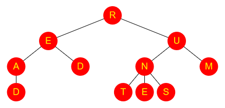
It looks like a real-life tree, only upside-down. Specifically:
- The “root” of the tree (at the top, in this case, “R”) has one or more “branches”
- Each of those branches has one or more branches
- And so on, until eventually a “leaf” is reached, i.e. a node with no branches coming off it
A common data structure is a binary tree, where each node has at most two branches. Typically data will be arranged in a binary tree as follows:
- Each node (root, branch or leaf) contains one piece of data
- The left branch contains all the data that is “less than” what’s in the parent node
- The right branch contains all the data that is “greater than” what’s in the parent node
Doing a search for a value in a binary tree is very similar to the binary search on a list discussed above, except that the tree structure is used to guide the search:
- Check the root node
- If this is the element being searched for, then the search is successful and the operation stops
- Otherwise, is the target element less than or greater than this one?
- If less than, repeat the algorithm but starting with the left branch
- Otherwise, repeat but starting with the right branch
The complexity of this search is generally the same as for binary search on a list (O(log n)), although this is contingent on the tree being reasonably well balanced. If the root node happens to have the greatest value, then there is no right branch and only a left branch – in the worst case, if the tree is similarly unbalanced all the way down, it might be necessary to check every single node in the tree, i.e. much like a linear search.
Depth first and breadth first search
Consider the scenario of a tree data structure that is not ordered, or is ordered by something other than the field being searched on. There are two main strategies that can be used – depth first or breadth first.
Breadth first search involves checking the root node, and then checking all its children, and then checking all the root’s grandchildren, and so on. All the nodes at one level of the tree are checked before descending to the next level.
Depth first search, by contrast, involves checking all the way down one branch of the tree until a leaf is reached and then repeating for the next route down to a leaf, and so on. For example one can start by following the right branch every time, then going back and level and following the left branch instead, and so on.
The implementations of breadth first and depth first search are very similar. Here is some pseudocode for depth first search, using a Stack:
push the root node onto a stack
while (stack is not empty)
  pop a node off the stack
  check this node to see if it matches your search (if so, stop!)
  push all the children of this node onto the stack
Breadth first search is identical, except that instead of a Stack, a Queue is used. Work through a small example and check you can see why the Stack leads to a depth first search, while a Queue leads to breadth first.
Which approach is best depends on the situation. If the tree structure is fixed and of known size, but there is no indication of where the item being searched for lies, then it might be necessary to search the entire tree. In that case, breadth first and depth first will take exactly the same length of time. So the only pertinent question is how much memory will be used by the Stack / Queue – if the tree is wide but shallow, depth first will use less memory; if it’s deep but narrow, breadth first will be better. Obviously, if there is some knowledge of where the answer is most likely to lie, that might influence the search strategy chosen.
Searching through data that doesn’t exist yet
Depth first and breadth first search are quite straightforward when there is a regular data structure all loaded into memory at once. However, exactly the same approach can be used to explore a search space that needs to be calculated on the fly. For example, in a chess computer: the current state of the chessboard is known (the root of the tree), but the subsequent nodes will need to be computed as the game proceeds, based on the valid moves available at the time. The operation “push all the children of this node onto the stack (or queue)” involves calculating the possible moves. Since chess is a game with many possible moves, the tree will be very wide – so it may be preferable to do a depth first search (limiting the process to exploring only a few moves ahead) to avoid using too much memory. Or perhaps it would be preferable to do a breadth first search in order to quickly home in on which is the best first move to make; after all, if checkmate can be reached in one move, there’s no point exploring other possible routes.
Part 5 – Dictionaries and sets
The above sections explore how data may be stored in lists. This topic looks at the other most common class of data structures, storing unsorted collections and lookup tables. The goal of this section is to understand where to use a structure such as a dictionary or set, and enough about how they work internally to appreciate their performance characteristics and trade-offs.
Dictionaries or Maps
In modern programming languages, the term “map” is generally used as a synonym for “dictionary”. Throughout the rest of this topic, the word “dictionary” will be used for consistency.
A dictionary is like a lookup table. Given a key, one can find a corresponding value. For example, a dictionary could store the following mapping from employee IDs to employee names:
| Key | Value |
|---|---|
| 17 | Fred |
| 19 | Sarah |
| 33 | Janet |
| 42 | Matthew |
A dictionary typically has four key operations:
- Add a key and value to the dictionary
- Test whether a particular key exists
- Retrieve a value given its key
- Remove a key (and its value) from the dictionary
Dictionaries are very useful data structures because a lot of real-world algorithms involve looking up data rather than looping over data. Dictionaries allow you to pinpoint and retrieve a specific piece of information, rather than having to scan through a long list.
Dictionary implementations
Almost any programming language will have one or more dictionaries in its base class library. For example in C# the IDictionary<TKey,TValue> interface describes a dictionary supporting all three operations above (Add, ContainsKey, the array indexer dictionary[key], and Remove), and more. The Dictionary<TKey,TValue> class is the standard implementation of this interface, although there are many more e.g. a SortedDictionary<TKey,TValue> which can cheaply return an ordered list of its keys.
It is worth understanding something about how dictionaries are implemented under the covers, so we will explore some options in the next few sections.
List dictionaries
The naive implementation of a dictionary is to store its contents as an array or list. This is fairly straightforward to implement and gives great performance for adding values to the dictionary (just append to the array). Typically a linked list would be used, which means that removing values is efficient too. Keys can also be easily retrieved in the order they’d been added, which may be useful in some situations.
However, list dictionaries are very expensive to do lookups in. The entire list must be iterated over in order to find the required key – an O(n) operation. Since this is normally a key reason for using a dictionaries, list dictionaries are relatively rarely the preferred choice.
C# used to provide a ListDictionary because it’s sometimes the fastest implementation for very small dictionaries, but its use is now highly discouraged; it hasn’t been updated to take advantage of generics and hence is significantly inferior to Dictionary<TKey,TValue>.
Hash tables
One of the fastest structures for performing lookups is a hash table. This is based around computing a hash for each object – a function that returns (typically) an integer.
- Create an array of ‘buckets’
- Compute the hash of each object, and place it in the corresponding bucket
Picking the right number of buckets isn’t easy – if there are too many then a lot of unnecessary space will be used, but if there are too few then there will be large buckets that take more time to search through.
The algorithm for looking up an object is:
- Compute the hash of the desired object
- Look up the corresponding bucket. How this is done is left up to the language implementation but is guaranteed to have complexity
O(1); a naive approach would be to use the code as a memory address offset - Search through the bucket for the object
Since looking up the bucket is a constant O(1) operation, and each bucket is very small (effectively O(1)), the total lookup time is O(1).
C#’s Dictionary<TKey,TValue> class is implemented using hash tables. Usually the generic type TKey’s own GetHashCode() and Equals() methods are used for steps 1. & 3. above, although the Dictionary constructor can be given an implementation of IEqualityComparer<T> that provides the methods.
Sets
Like the mathematical concept, a set is an unordered collection of unique elements.
You might notice that the keys of a dictionary or map obey very similar rules – and in fact, any dictionary/map can be used as a set by ignoring the values.
The main operations on a set are:
- Add – Add an item to the set (duplicates are not allowed)
- Contains – Check whether an item is in the set
- Remove – Remove an item from the set
These operations are similar to those on a list, but there are situations where a set is more appropriate:
- A set enforces uniqueness
- A set is generally optimised for lookups (it generally needs to be, to help it ensure uniqueness), so it’s quick to check whether something’s in the set
- A set is explicitly unordered, and it’s worth using when there is a need to add/remove items but the order is irrelevant – by doing so, it is explicit to future readers or users of the code about what is needed from the data structure
Because of their similarities to Dictionaries, the implementations are also very similar – in C# the standard implementation of ISet<T> is HashSet<T> (though there are other more specialised implementations, like SortedSet<T>).