Databases
- Understanding how to use relational and non-relational databases
- Linking code to datasets
Relational Databases, and in particular SQL (Structured Query Language) databases, are a key part of almost every application. You will have seen several SQL databases earlier in the course, but this guide gives a little more detail.
Most SQL databases work very similarly, but there are often subtle differences between SQL dialects. This guide will use MySQL for the examples, but these should translate across to most common SQL databases.
The MySQL Tutorial gives an even more detailed guide, and the associated reference manual will contain specifications for all MySQL features.
CREATE DATABASE cat_shelter;
Tables and Relationships
In a relational database, all the data is stored in tables, for example we might have a table of cats:
| id | name | age |
|---|---|---|
| 1 | Felix | 5 |
| 2 | Molly | 3 |
| 3 | Oscar | 7 |
Each column has a particular fixed type. In this example, id and age are integers, while name is a string.
The description of all the tables in a database and their columns is called the schema of the database.
Creating Tables
The scripting language we use to create these tables is SQL (Structured Query Language) – it is used by virtually all relational databases. Take a look at the CREATE TABLE command:
CREATE TABLE cats (
   id INT NOT NULL AUTO_INCREMENT PRIMARY KEY,
   name VARCHAR(255) NULL,
   age INT NOT NULL
);
This means
- Create a table called
cats - The first column is called
id, has typeint(integer), which may not be null, and forms an auto-incrementing primary key (see below) - The second column is called
name, has typevarchar(255)(string with max length 255), which may be null - The third column is called
age, has typeint(integer), which may not be null
You can use the mysql command-line to see all tables in a database – use the show tables command:
mysql-sql> show tables;
+-----------------------+
| Tables_in_cat_shelter |
+-----------------------+
| cats                  |
+-----------------------+
To see the schema for a particular table, you can use the describe command:
mysql-sql> describe cats;
+-------+--------------+------+-----+---------+----------------+
| Field | Type         | Null | Key | Default | Extra          |
+-------+--------------+------+-----+---------+----------------+
| id    | int(11)      | NO   | PRI | null    | auto_increment |
| name  | varchar(255) | YES  |     | null    |                |
| age   | int(11)      | NO   |     | null    |                |
+-------+--------------+------+-----+---------+----------------+
In MySQL workbench, you can also inspect the schema using the GUI.
Primary Keys
The Primary Key for a table is a unique identifier for rows in the table. As a general rule, all tables should have a primary key. If your table represents a thing then that primary key should generally be a single unique identifier; mostly commonly that’s an integer, but in principle it can be something else (a globally unique ID (GUID), or some “natural” identifier e.g. a users table might have a username that is clearly unique and unchanging).
If you have an integer primary key, and want to automatically assign a suitable integer, the AUTO_INCREMENT keyword will do that – the database will automatically take the next available integer value when a row is inserted (by default starting from 1 and incrementing by 1 each time).
When writing SELECT statements, any select by ID should be checked in each environment (staging, uat, production etc.) as an auto increment ID field cannot be relied upon to be correct across multiple environments.
Foreign Keys
Suppose we want to add a new table for owners. We need to create the owners table, but also add an owner_id column to our cats table:
CREATE TABLE owners (
    id INT NOT NULL AUTO_INCREMENT PRIMARY KEY,
    name VARCHAR(255) NOT NULL
);

ALTER TABLE cats
    ADD owner_id INT NOT NULL,
    ADD FOREIGN KEY (owner_id) REFERENCES owners (id);
The first block should be familiar, the second introduces some new things
- Alter the
catstable - Add a new column called
owner_id, which has typeintand is not null - Add a foreign key on the
owner_idcolumn, referencingowners.id
A foreign key links two fields in different tables – in this case enforcing that owner_id always matches an id in the owners table. If you try to add a cat without a matching owner_id, it will produce an exception:
mysql-sql> INSERT INTO cats (name, age, owner_id) VALUES ('Felix', 3, 543);
Error Code: 1452. Cannot add or update a child row: a foreign key constraint fails (cat_shelter.cats, CONSTRAINT cats_ibfk_1 FOREIGN KEY (owner_id) REFERENCES owners (id))
Using keys and constraints is very important – it means you can rely on the integrity of the data in your database, with almost no extra work!
Querying data
Defining tables, columns and keys uses the Data Definition Language (DDL), working with data itself is known as Data Manipulation Language (DML). Usually you use DDL when setting up your database, and DML during the normal running of your application.
Inserting data
To start off, we need to insert data into our database using the INSERT statement. This has two common syntaxes:
-- Standard SQL syntax
INSERT INTO cats (name, age, owner_id) VALUES ('Oscar', 3, 1), ('Molly', 5, 2);

-- MySQL extension syntax
INSERT INTO cats SET name='Felix', age=3, owner_id=1;
Note that:
- The double dash, --, starts a comment
- Multiple inserts can be performed at once, by separating the value sets
- The
AUTO_INCREMENTid field does not need to be specified
Selecting data
Now we’ve got some data, we want to SELECT it. The most basic syntax is:
SELECT <list_of_columns> FROM <name_of_my_table> WHERE <condition>;
For example, to find cats owned by owner 3:
SELECT name FROM cats WHERE owner_id = 3;
Some extra possibilities:
- You can specify
*for the column list to select every column in the table:SELECT * FROM cats WHERE id = 4; - You can omit the condition to select every row in the table:
SELECT name FROM cats; - You can perform arithmetic, and use
ASto output a new column with a new name (this column will not be saved to the database):SELECT (4 * age + 16) AS age_in_human_years FROM cats;
Ordering and Paging
Another common requirement for queried data is ordering and limiting – this is particularly useful for paging through data. For example, if we’re displaying cats in pages of 10, to select the third page of cats we can use the ORDER BY, OFFSET and LIMIT clauses:
SELECT * FROM cats ORDER BY name DESC LIMIT 10 OFFSET 20;
This will select cats:
- Ordered by
namedescending - Limited to 10 results
- Skipping the first 20 results
Performing these operations in the database is likely to be much faster than fetching the data and attempting to sort and paginate the data in the application. Databases are optimised for these kinds of tasks!
Updating data
This uses the UPDATE statement:
UPDATE <table> SET <column> = <value> WHERE <condition>
As a concrete example, let’s say we want to rename cat number 3:
UPDATE cats SET name = 'Razor' WHERE id = 3;
You can update multiple values by comma separating them, and even update multiple tables (but make sure to specify the columns explicitly).
Some SQL dialects allow you to perform an ‘upsert’ – updating an entry or inserting it if not present. In MySQL this is INSERT ... ON DUPLICATE KEY UPDATE. It looks a little bit like:
INSERT INTO mytable (id, foo) VALUES (1, 'bar')
ON DUPLICATE KEY UPDATE foo = 'bar';
But be careful – this won’t work in other dialects!
MySQL allows you to SELECT some data from a second table while performing an UPDATE, for example here we select the owners table:
UPDATE cats, owners
  SET cats.name = CONCAT(owners.name, '\'s ', cats.name)
  WHERE owners.id = cats.owner_id;
CONCAT is the SQL function used to concatenate strings.
This is actually a simplified form of an even more general style of query. Here we add the owners name to the cats name, but only when the owners name is not an empty string:
UPDATE cats, (SELECT name, id FROM owners WHERE name != "") AS named_owners
  SET cats.name = CONCAT(named_owners.name, '\'s ', cats.name)
  WHERE named_owners.id = cats.owner_id;
Deleting data
Use a DELETE query to delete data.
DELETE FROM cats WHERE id = 8;
You can omit the condition, but be careful – this will delete every row in the table!
Data Types
There are a large number of data types, and if in doubt you should consult the full reference. Some of the key types to know about are:
Numeric Types:
INT– a signed integerFLOAT– a single-precision floating point numberDOUBLE– a double-precision floating point numberDECIMAL– an ‘exact’ floating point numberBOOLEAN– secretly an alias for theTINYINT(1)type, which has possible values 0 and 1
String Types:
VARCHAR– variable length string, usually used for (relatively) short stringsTEXT– strings up to 65KB in size (useMEDIUMTEXTorLONGTEXTfor larger strings)BLOB– not really a string, but stores binary data up to 65KB (useMEDIUMBLOBorLARGEBLOBfor larger data)ENUM– a value that can only take values from a specified list
DateTime Types:
TIMESTAMP– an instant in time, stored as milliseconds from the epoch and may take values from1970-01-01to2038-01-19DATE– a date, as in'1944-06-06'TIME– a time, as in'23:41:50.1234'DATETIME– a combination of date and time
Almost all of these types allow specification of a precision or size – e.g. VARCHAR(255) is a string with max length of 255, a DATETIME(6) is a datetime with 6 decimal places of precision (i.e. microseconds).
NULL
Unless marked as NOT NULL, any value may also be NULL, however this is not simply a special value – it is the absence of a value. In particular, this means you cannot compare to NULL, instead you must use special syntax:
SELECT * FROM cats WHERE name IS NULL;
This can catch you out in a few other places, like aggregating or joining on fields that may be Null. For the most part, Null values are simply ignored and if you want to include them you will need to perform some extra work to handle that case.
Joins
The real power behind SQL comes when joining multiple tables together. The simplest example might look like:
SELECT owners.name AS owner_name, cats.name AS cat_name
  FROM cats INNER JOIN owners ON cats.owner_id = owners.id;
This selects each row in the cats table, then finds the corresponding row in the owners table – ‘joining’ it to the results.
- You may add conditions afterwards, just like any other query
- You can perform multiple joins, even joining on the same table twice
The join condition (cats.owner_id = owners.id in the example above) can be a more complex condition – this is less common, but can sometimes be useful when selecting a less standard data set.
There are a few different types of join to consider, which behave differently. Suppose we have two tables, left and right – we want to know what happens when the condition matches.
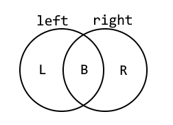
In the above, ‘L’ is the set of rows where the left table contains values but there are no matching rows in right, ‘R’ is the set of rows where the right table contains values but not the left, and ‘B’ is the set of rows where both tables contain values.
| Join Type | L | B | R |
|---|---|---|---|
INNER JOIN (or simply JOIN) |  |  | |
LEFT JOIN | | | |
RIGHT JOIN | | | |
Left and right joins are types of ‘outer join’, and when rows exist on one side but not the other the missing columns will be filled with NULLs. Inner joins are most common, as they only return ‘complete’ rows, but outer joins can be useful if you want to detect the case where there are no rows satisfying the join condition.
Always be explicit about the type of join you are using – that way you avoid any potential confusion.
Cross Joins
There’s one more important type of join to consider, which is a CROSS JOIN. This time there’s no join condition (no ON clause):
SELECT cats.name, owners.name FROM cats CROSS JOIN owners;
This will return every possible combination of cat + owner name that might exist. It makes no reference to whether there’s any link in the database between these items. If there are 4 cats and 3 owners, you’ll get 4 * 3 = 12 rows in the result. This isn’t often useful, but it can occasionally provide some value especially when combined with a WHERE clause.
A common question is why you need to specify the ON in a JOIN clause, given that you have already defined foreign key relationships on your tables. These are in fact completely different concepts:
- You can
JOINon any column or columns – there’s no requirement for it to be a foreign key. So SQL Server won’t “guess” the join columns for you – you have to state them explicitly. - Foreign keys are actually more about enforcing consistency – SQL Server promises that links between items in your database won’t be broken, and will give an error if you attempt an operation that would violate this.
Aggregates
Another common requirement is forming aggregates of data. The most common is the COUNT aggregate:
SELECT COUNT(*) FROM cats;
This selects a single row, the count of the rows matching the query – in this case all the cats. You can also add conditions, just like any other query.
MySQL includes a lot of other aggregate operations:
SUM– the sum of valuesAVG– the average (mean) of valuesMAX/MIN– the maximum/minimum of values
These operations ignore NULL values.
Grouping
When calculating aggregates, it can often be useful to group the values and calculate aggregates across each group. This uses the GROUP BY clause:
SELECT owner_id, COUNT(*) FROM cats GROUP BY owner_id;
This groups the cats by their owner_id, and selects the count of each group:
mysql-sql> SELECT owner_id, count(*) FROM cats GROUP BY owner_id;
+----------+----------+
| owner_id | count(*) |
+----------+----------+
|        1 |        2 |
|        2 |        4 |
|        3 |        1 |
+----------+----------+
You could also calculate several aggregates at once, or include multiple columns in the grouping.
You should usually include all the columns in the GROUP BY in the selected column list, otherwise you won’t know what your groups are!
Conversely, you should make sure every selected column is either an aggregate, or a column that is listed in the GROUP BY clause – otherwise it’s not obvious what you’re selecting.
Combining all these different types of query can get pretty complex, so you will likely need to consult the documentation when dealing with larger queries.
Stored Procedures
A “stored procedure” is roughly speaking like a function, it captures one or more SQL statements that you wish to execute in turn. Here’s a simple example:
CREATE PROCEDURE annual_cat_age_update ()
	UPDATE cats SET age = age + 1;
Now you just need to execute this stored procedure to increment all your cat ages:
CALL annual_cat_age_update;
Stored procedures can also take parameters (arguments). Let’s modify the above procedure to affect only the cats of a single owner at a time:
DROP PROCEDURE IF EXISTS annual_cat_age_update;

CREATE PROCEDURE annual_cat_age_update (IN owner_id int)
  UPDATE cats SET age = age + 1 WHERE cats.owner_id = owner_id;

CALL annual_cat_age_update(1);
There’s a lot more you can do with stored procedures – SQL is a fully featured programming language complete with branching and looping structures, variables etc. However in general it’s a bad idea to put too much logic in the database – the business logic layer of your application is a much better home for that sort of thing. The database itself should focus purely on data access – that’s what SQL is designed for, and it rapidly gets clunky and error-prone if you try to push it outside of its core competencies. This course therefore doesn’t go into further detail on more complex SQL programming – if you need to go beyond the basics, here is a good tutorial.
Locking and Transactions
Typically you’ll have many users of your application, all working at the same time, and trying to avoid them treading on each others’ toes can become increasingly more difficult. For example you wouldn’t want two users to take the last item in a warehouse at the same time. One of the other big attractions of using a database is built-in support for multiple concurrent operations.
Locking
The details of how databases perform locking isn’t in the scope of this course, but it can occasionally be useful to know the principle.
Essentially, when working on a record or table, the database will acquire a lock, and while a record or table is locked it cannot be modified by any other query. Any other queries will have to wait for it!
In reality, there are a lot of different types of lock, and they aren’t all completely exclusive. In general the database will try to obtain the weakest lock possible while still guaranteeing consistency of the database.
Very occasionally a database can end up in a deadlock – i.e. there are two parallel queries which are each waiting for a lock that the other holds. MySQL is usually able to detect this and one of the queries will fail.
Transactions
A closely related concept is that of transactions. A transaction is a set of statements which are bundled into a single operation which either succeeds or fails as a whole.
Any transaction should fullfil the ACID properties, these are as follows:
- Atomicity – All changes to data should be performed as a single operation; either all changes are carried out, or none are.
- Consistency – A transaction will never violate any of the database’s constraints.
- Isolation – The intermediate state of a transaction is invisible to other transactions. As a result, transactions that run concurrently appear to be running one after the other.
- Durability – Once committed, the effects of a transaction will persist, even after a system failure.
By default MySQL runs in autocommit mode – this means that each statement is immediately executed its own transaction. To use transactions, either turn off that mode or create an explicit transaction using the START TRANSACTION syntax:
START TRANSACTION;
UPDATE accounts SET balance = balance - 5 WHERE id = 1;
UPDATE accounts SET balance = balance + 5 WHERE id = 2;
COMMIT;
You can be sure that either both statements are executed or neither.
- You can also use
ROLLBACKinstead ofCOMMITto cancel the transaction. - If a statement in the transaction causes an error, the entire transaction will be rolled back.
- You can send statements separately, so if the first statement in a transaction is a
SELECT, you can perform some application logic before performing an UPDATE*
*If your isolation level has been changed from the default, you may still need to be wary of race conditions here.
If you are performing logic between statements in your transaction, you need to know what isolation level you are working with – this determines how consistent the database will stay between statements in a transaction:
READ UNCOMMITTED– the lowest isolation level, reads may see uncommitted (‘dirty’) data from other transactions!READ COMMITTED– each read only sees committed data (i.e. a consistent state) but multiple reads may return different data.REPEATABLE READ– this is the default, and effectively produces a snapshot of the database that will be unchanged throughout the entire transactionSERIALIZABLE– the highest isolation level, behaves as though all the transactions are performed in series.
In general, stick with REPEATABLE READ unless you know what you are doing! Increasing the isolation level can cause slowness or deadlocks, decreasing it can cause bugs and race conditions.
It is rare that you will need to use the transaction syntax explicitly.
Most database libraries will support transactions naturally.
Indexes and Performance
Data in a table is stored in a structure indexed by the primary key. This means that:
- Looking up a row by the primary key is very fast
- Looking up a row by any other field is (usually) slow
For example, when working with the cat shelter database, the following query will be fast:
SELECT * FROM cats WHERE id = 4
While the following query will be slow – MySQL has to scan through the entire table and check the age column for each row:
SELECT * FROM cats WHERE age = 3
The majority of SQL performance investigations boil down to working out why you are performing a full table scan instead of an index lookup.
The data structure is typically a B-Tree, keyed using the primary key of the table. This is a self-balancing tree that allows relatively fast lookups, sequential access, insertions and deletions.
Data is often stored in pages of multiple records (typically 8KB) which must all be loaded at once, this can cause some slightly unexpected results, particularly with very small tables or non-sequential reads.
Indexes
The main tool in your performance arsenal is the ability to tell MySQL to create additional indexes for a table, with different keys.
In a database context, the plural of index is typically indexes. In a mathematical context you will usually use indices.
Let’s create an index on the age column:
CREATE INDEX cats_age ON cats (age)
This creates another data structure which indexes cats by their age. In particular it provides a fast way of looking up the primary key (id) of a cat with a particular age.
With the new index, looking up a cat by age becomes significantly quicker – rather than scanning through the whole table, all we need to do is the following:
- A non-unique lookup on the new index –
cats_age - A unique lookup on the primary key –
id
MySQL workbench contains a visual query explainer which you can use to analyse the speed of your queries.
Try and use this on a realistic data set, as queries behave very differently with only a small amount of data!
You are not limited to using a single column as the index key; here is a two column index:
CREATE INDEX cats_age_owner_id ON cats (age, owner_id)
The principle is much the same as a single-column index, and this index will allow the query to be executed very efficiently by looking up any given age + owner combination quickly.
It’s important to appreciate that the order in which the columns are defined is important. The structure used to store this index will firstly allow MySQL to drill down through cat ages to find age = 3. Then within those results you can further drill down to find owner_id = 5. This means that the index above is has no effect for the following query:
SELECT * FROM cats WHERE owner_id = 5
Choosing which indexes to create
Indexes are great for looking up data, and you can in principle create lots of them. However you do have to be careful:
- They take up space on disk – for a big table, the index could be pretty large too
- They need to be maintained, and hence slow down
UPDATEandINSERToperations – every time you add a row, you also need to add an entry to every index on the table
In general, you should add indexes when you have reason to believe they will make a big difference to your performance (and you should test these assumptions).
Here are some guidelines you can apply, but remember to use common sense and prefer to test performance rather than making too many assumptions.
-
Columns in a foreign key relationship will normally benefit from an index, because you probably have a lot of
JOINs between the two tables that the index will help with. Note that MySQL will add foreign key indexes for you automatically. -
If you frequently do range queries on a column (for example, “find all the cats born in the last year”), an index may be particularly beneficial. This is because all the matching values will be stored adjacently in the index (perhaps even on the same page).
-
Indexes are most useful if they are reasonably specific. In other words, given one key value, you want to find only a small number of matching rows. If it matches too many rows, the index is likely to be much less useful.
Accessing databases through code
This topic discusses how to access and manage your database from your application level code.
The specific Database Management System (DBMS) used in examples below is MySQL, but most database access libraries will work with all mainstream relational databases (Oracle, Microsoft SQL Server, etc.). The same broad principles apply to database access from other languages and frameworks.
You should be able to recall using an Object Relational Mapper (ORM), Flask-SQLAlchemy, in the Bookish exercise and Whale Spotting mini-project; this topic aims to build on that knowledge and discuss these ideas in a more general, language-agnostic manner. For this reason, any code examples given will be in psuedocode.
Direct database access
At the simplest level, you can execute SQL commands directly from your application.
Exactly how this is done will depend on the tech stack you are using. In general, you must configure a connection to a specific database and then pass the query you wish to execute as a string to a query execution function.
For example, assuming we have a database access library providing connect_to_database and execute_query functions, some direct access code for the cat database might look something like this:
database_connection = connect_to_database(database_url, user, password)
query = "SELECT name FROM cats WHERE age > 4"
result = execute_query(database_connection, query)
Migrations
Once you’re up and running with your database, you will inevitably need to make changes to it. This is true both during initial development of an application, and later on when the system is live and needs bug fixes or enhancements. You can just edit the tables directly in the database – adding a table, removing a column, etc. – but this approach doesn’t work well if you’re trying to share code between multiple developers, or make changes that you can apply consistently to different machines (say, the test database vs the live database).
A solution to this issue is migrations. The concept is that you define your database changes as a series of scripts, which are run on any copy of the database in sequence to apply your desired changes. A migration is simply an SQL file that defines a change to your database. For example, your initial migration may define a few tables and the relationships between them, the next migration may then populate these tables with sample data.
There are a variety of different migration frameworks on offer that manage this proccess for you – you should remember using Flask-Migrate with Alembic in the Bookish exercise.
Each migration will have a unique ID, and this ID should impose an ordering on the migrations. The migration framework will apply all your migrations in sequence, so you can rely on previous migrations having happened when you write future ones.
Migrations also allow you to roll back your changes if you change your mind (or if you release a change to the live system and it doesn’t work…). Remember that this is a destructive operation – don’t do it if you’ve already put some important information in your new tables!
Some, but not all, migration frameworks will attempt to deduce how to roll back your change based on the original migration. Always test rolling back your migrations as well as applying them, as it’s easy to make a mistake.
Access via an ORM
An ORM is an Object Relational Mapper. It is a library that sits between your database and your application logic, and handles the conversion of database rows into objects in your application.
For this to work, we need to define a class in our application code to represent each table in the database that you would like to query. For example, we would create a Cat class with fields that match up with the columns in the cats database table. We could use direct database access as above to fetch the data, and then construct the Cat objects ourselves, but it’s easier to use an ORM. The @Key in the below psuedocode simply tells our psuedo-ORM that this field is the primary key; this will be relevant later.
class Cat {
  @Key id : int
  name : string
  age : int
  dateOfBirth : datetime
  owner : Owner
}

class Owner {
  id : int
  name : string
}
To do this, we provide the ORM with a SQL-like query to fetch the locations, but “by magic” it returns an enumeration of Cat objects – no need to manually loop through the results of the query or create our own objects. Behind the scenes, the ORM is looking at the column names returned by the query and matching them up to the field names on the Cat class. Using an ORM in this way greatly simplifies your database access layer.
function get_all_cats() : List<Cat> {
  connection_string = ORM.create_conn_string(database_url, user, password)
  connection = ORM.connect_to_database(connection_string)
  return connection.execute_query("SELECT * FROM Cats JOIN Owners ON Cats.OwnerId = Owners.Id")
}
Building object hierarchies
In the database, each Cat has an Owner. So the Cat class in our application should have an instance of an Owner class.
When getting a list of Cats, our ORM is typically able to deduce that the any Owner-related columns in our SQL query should be mapped onto fields of an associated Owner object.
One thing to note here is that if several cats are owned by Jane, then simpler ORMs might not notice that each cat’s owner is the same Jane and should share a single Owner instance. This may or may not be okay depending on your application: make sure you check!
SQL parameterisation and injection attacks
ORMs allow us to use parameterised SQL – a SQL statement that includes a placeholder for the the values in a query, e.g. a cat’s ID, which is filled in by the DBMS before the query is executed.
function get_cat(id : string) : Cat {
  connection_string = ORM.create_conn_string(database_url, user, password)
  connection = ORM.connect_to_database(connection_string)
  return connection.query(
    "SELECT * FROM Cats JOIN Owners ON Cats.OwnerId = Owners.Id WHERE Cats.Id = @id", id
  )
}
What if, instead of using paramaterised SQL, we had built our own query with string concatenation?
return connection.query(
  "SELECT * FROM Cats JOIN Owners ON Cats.OwnerId = Owners.Id WHERE Cats.Id = " + id
)
The way we’ve written this is important. Let’s check out what the query looks like when the user inputs 2.
SELECT * FROM Cats JOIN Owners ON Cats.OwnerId = Owners.Id WHERE Cats.Id = 2
This would work nicely. But what if someone malicious tries a slightly different input… say 1; INSERT INTO cats (name, age, owner_id) VALUES ('Pluto', 6, 2); -- ? Well, our query would now look like this:
SELECT * FROM Cats JOIN Owners ON Cats.OwnerId = Owners.Id WHERE Cats.Id = 1;
INSERT INTO cats (name, age, owner_id) VALUES ('Pluto', 6, 2); --
The edit would complete as expected, but the extra SQL added by the malicious user would also be executed and a dog would slip in to our Cats table! Your attention is called to this famous xkcd comic:

Never create your own SQL commands by concatenating strings together. Always use the parameterisation options provided by your database access library.
Leaning more heavily on the ORM
Thus far we’ve been writing SQL commands, and asking the ORM to convert the results into objects. But most ORMs will let you go further than this, and write most of the SQL for you.
function get_cat(id : string) : Cat {
  connection_string = ORM.create_conn_string(database_url, user, password)
  connection = ORM.connect_to_database(connection_string)
  return connection.get<Cat>(id)
}
How do ORMs perform this magic? It’s actually pretty straightforward. The class Cat presumably relates to a table named either Cat or Cats – it’s easy to check which exists. If you were fetching all cats then it’s trivial to construct the appropriate SQL query – SELECT * FROM Cats. And we already know that once it’s got the query, ORMs can convert the results into Cat objects.
Being able to select a single cat is harder – most ORMs are not quite smart enough to know which is your primary key field, but many will all you to explicitly tell them by assigning an attribute to the relevant property on the class.
Sadly, many ORMs also aren’t quite smart enough to populate the Owner property automatically when getting a Cat, and it will remain null. In general you have two choices in this situation:
- Fill in the Owner property yourself, via a further query.
- Leave it null for now, but retrieve it automatically later if you need it. This is called “lazy loading”.
Lazy loading
It’s worth a quick aside on the pros and cons of lazy loading.
In general, you may not want to load all your data from the database up-front. If it is uncertain whether you’ll need some deeply nested property (such as the Cat’s Owner in this example), it’s perhaps a bit wasteful to do the extra database querying needed to fill it in. Database queries can be expensive. So even if you have the option to fully populate your database model classes up-front (eager loading), you might not want to.
However, there’s a disadvantage to lazy loading too, which is that you have much less control over when it happens – you need to wire up your code to automatically pull the data from the database when you need it, but that means the database access will happen at some arbitrary point in the future. You have a lot of new error cases to worry about – what happens if you’re half way through displaying a web page when you try lazily loading the data, and the database has now gone down? That’s an error scenario you wouldn’t have expected to hit. You might also end up with a lot of separate database calls, which is also a bad thing in general – it’s better to reduce the number of separate round trips to the database if possible.
So – a trade off. For simple applications it shouldn’t matter which route you use, so just pick the one that fits most naturally with your ORM (often eager loading will be simpler, although frameworks like Ruby on Rails automatically use lazy loading by default). But keep an eye out for performance problems or application complexity so you can evolve your approach over time.
The best resources for relatively simple frameworks are generally their documentation – good libraries include well-written documentation that show you how to use the main features by example.
Have a look at the docs for SQLAlchemy, Flask-SQLAlchemy, Flask-Migrate, and Alembic if you want to learn more.
Non-relational databases
Non-relational is a catch all term for any database aside from the relational, SQL-based databases which you’ve been studying so far. This means they usually lack one or more of the usual features of a SQL database:
- Data might not be stored in tables
- There might not be a fixed schema
- Different pieces of data might not have relations between them, or the relations might work differently (in particular, no equivalent for
JOIN).
For this reason, there are lots of different types of non-relational database, and some pros and cons of each are listed below. In general you might consider using a non-relational when you you don’t need the rigid structure of a relational database.
Think very carefully before deciding to use a non-relational database. They are often newer and less well understood than SQL, and it may be very difficult to change later on. It’s also worth noting that some non-relational database solutions do not provide ACID transactions, so are not suitable for applications with particularly stringent data reliabilty and integrity requirements.
You might also hear the term NoSQL to refer to these types of databases. NoSQL databases are, in fact, a subset of non-relational databases – some non-relational databases use SQL – but the terms are often used interchangeably.
Key Value Stores
In another topic you’ll look at the dictionary data structure, wherein key data is mapped to corresponding value data. The three main operations on a dictionary are:
get– retrieve a value given its keyput– add a key and value to the dictionaryremove– remove a value given its key
A key value store exposes this exact same API. In a key value store, as in a dictionary, retrieving an object using its key is very fast, but it is not possible to retrieve data in any other way (other than reading every single document in the store).
Unlike relational databases, key-value stores are schema-less. This means that the data-types are not specified in advance (by a schema).
This means you can often store binary data like images alongside JSON information without worrying about it beforehand. While this might seem powerful it can also be dangerous – you can no longer rely on the database to guarantee the type of data which may be returned, instead you must keep track of it for yourself in your application.
The most common use of a key value store is a cache; this is a component which stores frequently or recently accessed data so that it can be served more quickly to future users. Two common caches are Redis and Memcached – at the heart of both are key value stores kept entirely in memory for fast access.
Document Stores
Document stores require that the objects are all encoded in the same way. For example, a document store might require that the documents are JSON documents, or are XML documents.
As in a key value store, each document has a unique key which is used to retrieve the document from the store. For example, a document representing a blog post in the popular MongoDB database might look like:
{
  "_id": "5aeb183b6ab5a63838b95a13",
  "name": "Mr Burns",
  "email": "c.m.burns@springfieldnuclear.org",
  "content": "Who is that man?",
  "comments": [
    {
      "name": "Smithers",
      "email": "w.j.smithers@springfieldnuclear.org",
      "content": "That's Homer Simpson, sir, one of your drones from sector 7G."
    },
    {
     "name": "Mr Burns",
     "email": "c.m.burns@springfieldnuclear.org",
     "content": "Simpson, eh?"
    }
  ]
}
In MongoDB, the _id field is the key which this document is stored under.
Indexes in non-relational databases
Storing all documents with the same encoding allows documents stores to support indexes. These work in a similar way to relational databases, and come with similar trade-offs.
For example, in the blog post database you could add an index to allow you to look up documents by their email address and this would be implemented as a separate lookup table from email addresses to keys. Adding this index would make it possible to look up data via the email address very quickly, but the index needs to be kept in sync – which costs time when inserting or updating elements.
Storing relational data
The ability to do joins between tables efficiently is a great strength of relational databases such as MySQL and is something for which there is no parallel in a non-relational database. The ability to nest data mitigates this somewhat but can produce its own set of problems.
Consider the blog post above. Due to the nested comments, this would need multiple tables to represent in a MySQL databases – at least one for posts and one for comments, and probably one for users as well. To retrieve the comments shown above two tables would need to be joined together.
SELECT users.name, users.email, comments.content
  FROM comments
  JOIN users on users.id = comments.author
  WHERE comments.post = 1;
So at first sight, the document store database comes out on top as the same data can be retrieved in a single query without a join.
collection.findAll({_id: new ObjectId("5aeb183b6ab5a63838b95a13")})["comments"];
But what if you need to update Mr Burns’ email address? In the relational database this is an UPDATE operation on a single row but in the document store you may need to update hundreds of documents looking for each place that Mr Burns has posted, or left a comment! You might decide to store the users’ email addresses in a separate document store to mitigate this, but document stores do not support joins so now you need two queries to retrieve the data which previously only needed a single query.
Roughly speaking, document stores are good for data where:
- Every document is roughly similar but with small changes, making adding a schema difficult.
- There are very few relationships between other elements.
Sharding
Sharding is a method for distributing data across multiple machines, which is used when a single database server is unable to cope with the required load or storage requirements. The data is split up into ‘shards’ which are distributed across several different database servers. This is an example of horizontal scaling.
In the blog post database, we might shard the database across two machines by storing blog posts whose keys begin with 0-7 on one machine and those whose keys begin 8-F on another machine.
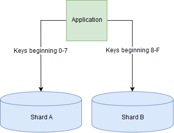
Sharding relational databases is very difficult, as it becomes very slow to join tables when the data being joined lives on more than one shard. Conversely, many document stores support sharding out of the box.
More non-relational databases
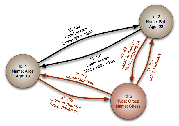
Graph databases are designed for data whose relationships fit into a graph, where graph is used in the mathematical sense as a collection of nodes connected by edges. For example a graph database could be well suited for a social network where the nodes are users and friend ships between users are modelled by edges in the graph. Neo4J is a popular graph database.
A distributed database is a database which can service requests from more than one machine, often a cluster of machines on a network.
A sharded database as described above is one type of this, where the data is split across multiple machines. Alternatively you might choose to replicate the same data across multiple machines to provide fault tolerance (if one machine goes offline, then not all the data is lost). Some distributed databases also offer guarantees about what happens if half of your database machines are unable to talk to the other half – called a network partition – and will allow some of both halves to continue to serve requests. With these types of databases, there are always trade-offs between performance (how quickly your database can respond to a request), consistency (will the database ever return “incorrect” data), and availability (will the database continue to serve requests even if some nodes are unavailable). There are numerous examples such as Cassandra and HBase, and sharded document stores including MongoDB can be used as distributed databases as well.
Further reading on non-relational databases
For practical further reading, there is a basic tutorial on how to use MongoDB from a NodeJS application on the W3Schools website.