Databases
- Understanding how to use relational and non-relational databases
- Linking code to datasets
This course is about databases. Most SQL (Structured Query Language) databases work very similarly, but there are often subtle differences between SQL dialects. This guide will use Microsoft SQL Server for the examples, but these should translate across to most common SQL databases.
The topics in this module contain enough information for you to get started. You might like to do some further reading beyond this though; we recommend the following resources:
- Book: SAMS Teach Yourself Transact-SQL in 21 Days. This is a good introductory reference to SQL, covering the version used by Microsoft SQL Server. You may find it useful as a reference book for looking up more detail on particular topics.
- Microsoft Virtual Academy: Querying Data with Transact-SQL provides a good grounding in everything necessary to extract data from SQL Server (including some topics that we don’t go into detail on here).
- Online tutorial: W3Schools SQL Tutorial. The W3Schools tutorial works through topics in a slightly different order from this module. Alternatively you might find it more useful to dip in and out of to explore particular topics – each page in the tutorial is quite standalone and you can jump straight to any section.
CREATE DATABASE cat_shelter;
Tables and Relationships
A database is an application that stores data, and tables are the structures within which data is stored; relationships are the links between tables.
Creating Tables
A table is a structure within the database that stores data. For example, suppose we are building a database for a cattery; we might have a table within this database called Cats which stores information about all the individual cats that are currently staying with us.
| id | name | age |
|---|---|---|
| 1 | Felix | 5 |
| 2 | Molly | 3 |
| 3 | Oscar | 7 |
Each column has a particular fixed type. In this example, id and age are integers, while name is a string.
The description of all the tables in a database and their columns is called the schema of the database.
The scripting language we use to create these tables is SQL (Structured Query Language) – it is used by virtually all relational databases, although there are subtle syntax differences between them. Take a look at the CREATE TABLE command:
CREATE TABLE Cats (
    Id Int IDENTITY NOT NULL PRIMARY KEY,
    Name nvarchar(max) NULL
)
This says:
- Create a table called
Cats - The first column should be called
Id, of typeint(integer), which must be filled in with a value (NOT NULL) - The second column should be called
Name, of typenvarchar(max)(string, with no particular length limit), which can be set toNULL
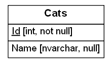
A graphical way to represent your database is an Entity Relationship (ER) Diagram – ours is currently very simple because we only have a single table:
Primary Keys
The Primary Key for a table is a unique identifier for rows in the table. As a general rule, all tables should have a primary key. If your table represents a thing then that primary key should generally be a single unique identifier; mostly commonly that’s an integer, but in principle it can be something else (a globally unique ID (GUID), or some “natural” identifier e.g. a users table might have a username that is clearly unique and unchanging).
In the ER diagram, the primary key is underlined. In the SQL CREATE TABLE statement, it’s marked with the keywords PRIMARY KEY. In SQL Server Management Studio you can see the primary key listed under “Keys” (it’s the one with an autogenerated name prefixed “PK”).
If you have an integer primary key, and want to automatically assign a suitable integer, the IDENTITY keyword in the SQL will do that – that means it will automatically take the next available integer value (by default starting from 1 and incrementing by 1 each time). SQL Server will assign a suitable value each time you create a row.
When writing SELECT statements, any select by ID should be checked in each environment (staging, uat, production etc.) as an auto increment ID field cannot be relied upon to be correct across multiple environments.
Relationships
Relational databases are all about the relationships between different pieces of data. In the case of cats, presumably each cat has an owner. We can enhance our Entity Relationship diagram to demonstrate this:
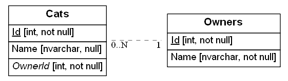
The relationship in the diagram is shown as “0..N to 1”. So one owner can have any number of cats, including zero. But every cat must have an owner. You can see that this one-to-many relationship is implicit in the fields in the database – the Cats table has an OwnerId column, which is not nullable, so each cat must have an owner; but there is no particular constraint to say whether an owner necessarily has a cat, nor any upper limit to how many cats an owner might have.
Foreign Keys
A foreign key links two fields in different tables – in this case enforcing that owner_id always matches an id in the owners table. If you try to add a cat without a matching owner_id, it will produce an exception:
sql> INSERT INTO cats (name, age, owner_id) VALUES ('Felix', 3, 543);
Error:. Cannot add or update a child row: a foreign key constraint fails (cat_shelter.cats, CONSTRAINT cats_ibfk_1 FOREIGN KEY (owner_id) REFERENCES owners (id))
Using keys and constraints is very important – it means you can rely on the integrity of the data in your database, with almost no extra work!
Joining Tables
We could enhance our database schema a bit more. Lets say our cattery is actually a national chain, and one of their selling points is keep-fit clubs for cats. Here’s our first attempt at the database design:
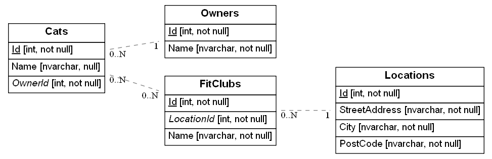
The interesting piece of the diagram is the link between Cats and FitClubs. Each Fit Club has zero or more Cats enrolled, and each Cat may be enrolled in zero or more Fit Clubs. Currently there’s nothing in the database to indicate which cats are in which fit club though – there are no suitable database fields. We can’t add a CatIdto FitClubs, because that would allow only a single cat to be a member; but nor can we add FitClubId to Catsas that would restrict us to at most one club per cat.
The solution is to introduce a joining table. It’s best to illustrate this explicitly in your ER diagram, as follows:
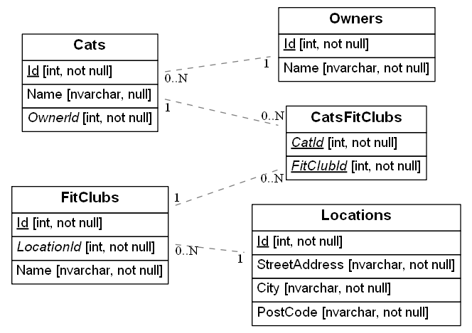
We’ve split the link from Cats to Fit Clubs by adding an extra table in the middle. Note that this table has a primary key (underlined fields) comprising of two columns – the combination of Cat ID and Fit Club ID makes up the unique identifier for the table. In general, relational databases can only allow one end of the relationship to feature many members; there needs to be one end that features at most a single row. Joining tables allow you to create many to many type relationships like the above.
It’s worth noting that joining tables can often end up being useful for more than just making the relationship work out. For example in this case it might be necessary to give each cat a separate membership number for each fit club they’re a member of; that membership number would make sense to live on the CatsFitClubs joining table.
Querying data
Defining tables, columns and keys uses the Data Definition Language (DDL), working with data itself is known as Data Manipulation Language (DML). Usually you use DDL when setting up your database, and DML during the normal running of your application.
Inserting data
We’ll start with inserting data into your database. This is done using the INSERT statement. The simplest syntax is this:
INSERT INTO name_of_my_table(list_of_columns) VALUES (list_of_values)
For example:
INSERT INTO Owners(Name) VALUES ('Fred')

INSERT INTO Cats(Name, OwnerId) VALUES ('Tiddles', 1)
Note that we don’t specify a value for the Id column in each case. This is because we defined it as an IDENTITY column – it will automatically be given an appropriate value. If you do try to assign a value yourself, it will fail. (If you ever need to set your own value, look up SET IDENTITY INSERT ON in the documentation. It’s occasionally valid to do this, but on the whole it’s best to let SQL Server deal with the identity column itself).
Selecting data
When we have some data, we want to SELECT it. The most basic syntax is:
SELECT list_of_columns FROM name_of_my_table WHERE condition
For example, let’s find the cats owned by owner #3:
SELECT Name FROM Cats WHERE OwnerId = 3
If this query is executed in SQL Server Management Studio, the results would look like this:
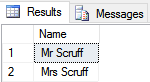
Note that what you get back is basically another table of data, but it has only the rows and columns that you asked for.
Here are some more things you can do with the list_of_columns. Try them all out:
- Select multiple columns.
SELECT Name, Age FROM Cats WHERE OwnerId = 3 - Select all columns.
SELECT * FROM Cats WHERE OwnerId = 3 - Perform calculations on columns.
SELECT Age * 4 FROM Cats WHERE OwnerId = 3(a naive attempt to return the age of the cat in human years. Sorry cat lovers, this is terribly inaccurate)
And here are some things you can do with condition:
- Use operators other than “=”.
SELECT Name FROM Cats WHERE Age > 2 - Use “AND” and “OR” to build more complex logic.
SELECT Name FROM Cats WHERE Age > 2 AND OwnerId = 2 - Omit it entirely.
SELECT Name FROM Cat
Ordering and Paging
Another common requirement for queried data is ordering and limiting – this is particularly useful for paging through data. For example, if we’re displaying cats in pages of 10, to select the third page of cats we can use the ORDER BY, OFFSET and LIMIT clauses:
SELECT * FROM cats ORDER BY name DESC LIMIT 10 OFFSET 20;
This will select cats:
- Ordered by
namedescending - Limited to 10 results
- Skipping the first 20 results
Performing these operations in the database is likely to be much faster than fetching the data and attempting to sort and paginate the data in the application. Databases are optimised for these kinds of tasks!
Updating data
There’s a lot more we can do with querying data, but for now we’ll move on to modifying data in a database. This is done using the UPDATE statement:
UPDATE name_of_my_table SET column = new_value WHERE condition
For example, let’s suppose the owner of cat number 3 has thought better of the name Bunnikins:
UPDATE Cats SET Name = 'Razor' WHERE Id = 2
Here are some more things you can do with updates.
- Update multiple columns at once.
UPDATE Cats SET Name = 'Razor', OwnerId = 3 WHERE Id = 2 - Use columns from your table in the
SETclause.UPDATE Cats SET Name = Name + ' The Angry Cat' WHERE Id = 2(work out what you think it’ll do, then check) - Omit the
WHEREclause.UPDATE Cats SET Age = Age + 1(but be careful! This one might make sense, but missing out yourWHEREclause is a common cause of accidentally corrupting your entire database…) SELECTsome data from another table, and use that in yourSETclause.UPDATE Cats SET Name = Owners.Name + '''s ' + Cats.Name FROM Owners WHERE Owners.Id = Cats.OwnerId
That last example is a bit more complicated and merits a more detailed look. We’ll break it down a bit. Here’s another way of laying out the same query:
UPDATE Cats
SET Name = Owners.Name + '''s '+ Cats.Name
FROM Owners
WHERE Owners.Id = Cats.OwnerId
This means:
Update the Cats table as follows:
Set each cat's Name to be its Owner's Name, followed by 's, followed by its original name
Using a row from the Owners table
Where the Owner's ID is the Cat's OwnerId
There are some extra bits of syntax we’ve sneaked in that are worth drawing out more explicitly;
- The
'''s 'represents a string (strings in SQL are contained in single quotes:') containing a single quote, an s and a space. The single quote (') is doubled up ('') to stop SQL Server from thinking that you’re indicating the end of the string. - You can prefix any column with the name of its table (e.g.
Owners.Namein the above example). This is necessary in this case because there are two tables with aNamecolumn, and without spelling it out SQL Server can’t tell which name it’s supposed to use. (There’s one table name prefix in the example above that’s not strictly necessary. Can you see which?). Note that you always need to include the table in aFROMclause or equivalent – simply using its name as a prefix to a column name doesn’t magically make the table available.
Deleting data
Use a DELETE query to delete data.
DELETE Cats WHERE Name = 'Bill''s Old Faithful'
There WHERE clause works just like in the other types of query. And just like in those other cases, it’s optional – omitting it will attempt to delete everything in the table:
DELETE Cats
Fortunately in this case this command should fail (the foreign key relationships won’t let you delete a cat if it’s assigned to a fit club, and this will abort the entire statement). Just like with UPDATE, it’s important to be careful when running DELETEs as missing the WHERE clause out by accident could have disastrous consequences.
Inserting data based on a selection
As a final flourish, let’s revisit the INSERT statement now that we’ve covered all the other statement types. Previously we saw how to insert a single row into a table, with fixed values. But you can also combine INSERT with SELECT to insert many rows at a time, or insert based on values pulled out of the database. Let’s consider the second case first, and add an extra cat without needing to hard-code its owner’s ID:
INSERT INTO Cats(Name, OwnerId) SELECT 'Cuddles', Id FROM Owners WHERE Name = 'Jane'
If you ran just the SELECT part of that query, you’d see:
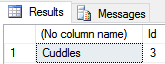
Adding the INSERT on the front just directs this data into a new row in the Cats table.
You can use the same principle to add multiple rows at once – just use a SELECT statement that returns multiple rows:
INSERT INTO Cats(Name, OwnerId) SELECT Name + '''s new cat', Id FROM Owners
Now everyone has a new cat.
Data Types
There are a large number of data types, and if in doubt you should consult the full reference. Some of the key types to know about are:
Numeric Types:
int– a signed integerfloat– a single-precision floating point numberdecimal– an ‘exact’ floating point numbermoney– to represent monetary values
String Types:
varchar– variable length string, usually used for (relatively) short stringstext– strings up to 65KB in size (useMEDIUMTEXTorLONGTEXTfor larger strings)binary– not really a string, but stores binary data up to 65KB
Dates and Times
Dates and times can be stored in SQL Server using the datetime data type. There’s no way to store “just” a time, although you could use a fixed date and just worry about the time part (if you pass just a time to SQL Server, it will assume you’re talking about 1st January 1900).
To add a date of birth column to the Cats table:
ALTER TABLE Cats

ADD DateOfBirth datetime NULL
And then to set the date of birth for all cats called Cuddles:
UPDATE Cats SET DateOfBirth = '2012-05-12' WHERE Name = 'Cuddles'
Note that we can give the date as a string, and SQL Server will automatically convert it to a datetime for storage. Note that as only the date is being set, the database sets the time to midnight, although we may well choose to ignore this when using the data ourselves.
It’s worth thinking a little about how you write your dates. The query above would also work with SET DateOfBirth = '12 May 2012' – SQL Server is fairly flexible when parsing date strings. However you need to take care; consider SET DateOfBirth = '12/05/2012'. If your database is set to expect UK English dates, this will work. But if it’s set to use US English dates, you’ll get 5th December instead of 12th May. Similarly your database could be set to a non-English language in which case using “12 May 2012” will no longer work. So best practice is always to use a non-ambiguous year-month-day format, with month numbers rather than names, so you don’t run into trouble when your database goes live in a different country (or just with different settings) from what you originally expected.
There are also a few useful date/time manipulation functions that you should be aware of:
DATEPART(part, date)– returns one part of thedate. Valid values forpartinclude:year,quarter,month,dayofyear,day,week(i.e. week number within the year),weekday(e.g. Monday),hour,minute,second. There’s also aDATENAMEfunction that’s similar but returns the text version e.g. “May” rather than “5”.DATEADD(part, amount, date)– adds a number of days, years, or whatever todate.parttakes the same values as above, andamounttells you how many of them to add.DATEDIFF(part, date1, date2)– reports the difference between two dates. Againparttakes the same values as above.GETDATE()– returns the current date and time. There’s alsoGETUTCDATE()if you want to find the time in the GMT timezone – regularGETDATEreturns the time in the server’s timezone.
By way of example, here are a couple of queries which calculate each cat’s age from its date of birth, and (rather approximately) vice versa:
UPDATE Cats SET Age = DATEDIFF(year, DateOfBirth, GETDATE()) WHERE DateOfBirth IS NOT NULL

UPDATE Cats SET DateOfBirth = DATEADD(year, -Age, GETDATE()) WHERE Age IS NOT NULL
NULL
Unless marked as NOT NULL, any value may also be NULL, however this is not simply a special value – it is the absence of a value. In particular, this means you cannot compare to NULL, instead you must use special syntax:
SELECT * FROM cats WHERE name IS NULL;
This can catch you out in a few other places, like aggregating or joining on fields that may be null. For the most part, null values are simply ignored and if you want to include them you will need to perform some extra work to handle that case.
Joins
The real power behind SQL comes when joining multiple tables together. The simplest example might look like:
SELECT Cats.Name AS [Cat Name], Owners.Name AS [Owner Name] FROM Cats
JOIN Owners ON Cats.OwnerId = Owners.Id
This selects each row in the cats table, then finds the corresponding row in the owners table – ‘joining’ it to the results.
- You may add conditions afterwards, just like any other query
- You can perform multiple joins, even joining on the same table twice!
The join condition (Cats.OwnerId = Owners.Id in the example above) can be a more complex condition – this is less common, but can sometimes be useful when selecting a less standard data set.
There are a few different types of join to consider, which behave differently. Suppose we have two tables, left and right – we want to know what happens when the condition matches.
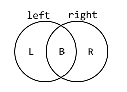
Where ‘L’ is the set of rows where the left table contains values but there are no matching rows in right, ‘R’ is the set of rows where the right table contains values but not the left, and ‘B’ is the set of rows where both tables contain values.
| Join Type | L | B | R |
|---|---|---|---|
INNER JOIN (or simply JOIN) |  |  | |
LEFT JOIN | | | |
RIGHT JOIN | | | |
Left and right joins are types of ‘outer join’, and when rows exist on one side but not the other the missing columns will be filled with NULLs. Inner joins are most common, as they only return ‘complete’ rows, but outer joins can be useful if you want to detect the case where there are no rows satisfying the join condition.
Always be explicit about the type of join you are using – that way you avoid any potential confusion.
Cross Joins
There’s one more important type of join to consider, which is a CROSS JOIN. This time there’s no join condition (no ON clause):
SELECT cats.name, owners.name FROM cats CROSS JOIN owners;
This will return every possible combination of cat + owner name that might exist. It makes no reference to whether there’s any link in the database between these items. If there are 4 cats and 3 owners, you’ll get 4 * 3 = 12 rows in the result. This isn’t often useful, but it can occasionally provide some value especially when combined with a WHERE clause.
A common question is why you need to specify the ON in a JOIN clause, given that you have already defined foreign key relationships on your tables. These are in fact completely different concepts:
- You can
JOINon any column or columns – there’s no requirement for it to be a foreign key. So SQL Server won’t “guess” the join columns for you – you have to state them explicitly. - Foreign keys are actually more about enforcing consistency – SQL Server promises that links between items in your database won’t be broken, and will give an error if you attempt an operation that would violate this.
Aggregates
Databases are good at performing data analysis tasks. It is worth understanding how to do this, because it is often more efficient to analyse data directly in the database than in a client application. (This is because the client application would have to download a lot of information from the database; that download is avoided if you do all the work on the database server).
The simplest analysis operation is to count the number of rows that match a query, with COUNT:
SELECT COUNT(*) FROM Cats WHERE OwnerId = 3
This query will return a single row – the COUNT aggregates (combines) all the rows that match the query and performs an operation on them, in this case counting how many of them there are.
SQL also includes other aggregate operations, for example
- Adding up a load of values.
SELECT SUM(Age) FROM Cats(although why you’d want to add up their ages, I don’t know…) - Finding an average.
SELECT AVG(Age) FROM Cats - Finding the smallest value.
SELECT MIN(Age) FROM Cats(MAXis available similarly) - Counting the number of unique values.
SELECT COUNT(DISTINCT OwnerId) FROM Cats(the number of different owners who have cats)
Grouping
The examples above work on an entire table, or all the results matching a WHERE clause. Aggregates are more powerful when combined with the GROUP BY clause. Consider the following:
SELECT MAX (Age), OwnerId FROM Cats GROUP BY OwnerId
This returns one row per owner in the database, and for each one it reports the age of their oldest cat.
Here are some more examples of aggregating data:
- Include more than one column in the
GROUP BY:SELECT COUNT(DISTINCT Name), OwnerId, Age FROM Cats GROUP BY OwnerId, Age- “For each owner and age of cat, count the number of unique names” – in real life, you’d hope there was only one…
- Calculate more than one aggregate at once:
SELECT COUNT(*), MAX(Age), OwnerId FROM Cats GROUP BY OwnerId- “For each owner, count the number of cats, and also the age of the oldest cat”
Basically GROUP BY X says “return one row for each value of column X”. This means:
- Every column referenced in the
SELECTmust either be aggregated, or be listed in theGROUP BY. Otherwise SQL Server doesn’t know what to do if the rows being aggregated take different values for that field. For example, imagine what you’d want to happen if you ran the invalidSELECT Name, MAX(Age), OwnerId FROM Cats GROUP BY OwnerId. You’d get only one row for each owner – what gets displayed in the row for owner 3, who has three cats all with different names? - You normally want to list every column that’s in the
GROUP BYclause in theSELECTclause too. But this isn’t mandatory.
Subqueries
It can sometimes be useful to use the results of one query within another query. This is called a subquery.
In general you can use a query that returns a single value anywhere that you could use that value. So for example:
SELECT Name, (SELECT Name FROM Owners WHERE Id = OwnerId) FROM Cats
This is valid, although you could express it much more clearly by using a JOIN onto the Owners table instead of a subquery. The rule in situations like this is that there must be only a single value from the query. The following should fail because some owners have several cats:
SELECT Name, (SELECT Name FROM Cats WHERE Owners.Id = OwnerId) FROM Owners
Since subqueries can be used anywhere that a normal value can be used, they can also feature in WHERE clauses:
SELECT * FROM Cats WHERE OwnerId = (SELECT Id FROM Owners WHERE Name = 'Jane')
Again this could be better expressed using a JOIN, but the flexibility can sometimes be useful.
In certain contexts, subqueries can be used even if they return multiple values. The most common is EXISTS – this is a check that can be used in a WHERE clause to select rows where a subquery returns at least one value. For example, this will select all owners who have at least one cat:
SELECT * FROM Owners WHERE EXISTS (SELECT * FROM Cats WHERE OwnerId = Owners.Id)
This allows us to revisit the code discussed under CROSS JOIN above that assigns cats to fit clubs. The first attempt looks like this:
INSERT INTO CatsFitClubs (CatId, FitClubId)
SELECT Cats.Id, FitClubs.Id
FROM Cats
CROSS JOIN FitClubs
This would fail – you can’t create duplicate (Cat, Fit Club) combinations. (This is enforced because CatId, FitClubId is the primary key). But you can use WHERE NOT EXISTS to remove those duplicates:
INSERT INTO CatsFitClubs (CatId, FitClubId)
SELECT Cats.Id, FitClubs.Id
FROM Cats
CROSS JOIN FitClubs
WHERE NOT EXISTS
  (SELECT *
  FROM CatsFitClubs
  WHERE CatId  = Cats.Id
  AND FitClubId = FitClubs.Id)
Subqueries can also be used in an IN clause, as follows:
SELECT * FROM Cats WHERE OwnerId IN (SELECT Id FROM Owners WHERE Name != 'Jane')
This probably isn’t the best way to write this particular query (can you find a better one, without IN?), but it illustrates the point – the subquery must return a single column, but can return many rows; cats will be selected if their owner is anywhere in the list provided by the subquery. Note that you can also hard-code your IN list – SELECT * FROM Cats WHERE OwnerId IN (1, 2). And there’s a NOT IN, which works just as you’d expect.
Views
A view is like a virtual table – you can use it in a SELECT statement just like a real table, but instead of having data stored in it, when you look at it it evaluates some SQL and returns the results. As such it’s a convenient shorthand for a chunk of SQL that you might need to use in multiple places – it helps you keep your SQL code DRY. (DRY = Don’t Repeat Yourself).
Create a view like this:
CREATE VIEW CatsWithOwners As
SELECT Cats.*, Owners.Name AS OwnerName
FROM Cats
JOIN Owners
ON Cats.OwnerId = Owners.Id
Now you can use it just as you would a table:
SELECT * FROM CatsWithOwners WHERE OwnerName = 'Jane'
Once you’ve created a view, if you want to change it you’ll either need to delete it and recreate it (DROP VIEW CatsWithOwners), or modify the existing definition (replace CREATE with ALTER in the code example above).
Stored Procedures
A stored procedure is roughly speaking like a method in a language like C# or Java. It captures one or more SQL statements that you wish to execute in turn. Here’s a simple example:
CREATE PROCEDURE AnnualCatAgeUpdate
AS
UPDATE Cats
SET Age = Age + 1
Now you would just need to execute this stored procedure to increment all your cat ages:
EXEC AnnualCatAgeUpdate
Stored procedures can also take parameters (arguments). Let’s modify the above procedure to affect only the cats of a single owner at a time:
ALTER PROCEDURE AnnualCatAgeUpdate
@OwnerId int
AS
UPDATE Cats
SET Age = Age + 1
WHERE OwnerId = @OwnerId
GO

EXEC AnnualCatAgeUpdate @OwnerId = 1
There’s a lot more you can do with stored procedures – SQL is a fully featured programming language complete with branching and looping structures, variables etc. However in general it’s a bad idea to put too much logic in the database – the business logic layer of your C# / Java application is a much better home for that sort of thing. The database itself should focus purely on data access – that’s what SQL is designed for, and it rapidly gets clunky and error-prone if you try to push it outside of its core competencies.
Locking
Typically you’ll have many users of your application, all working at the same time, and trying to avoid them treading on each others’ toes can become increasingly more difficult. For example you wouldn’t want two users to take the last item in a warehouse at the same time. One of the other big attractions of using a database is built-in support for multiple concurrent operations.
The details of how databases perform locking isn’t in the scope of this course, but it can occasionally be useful to know the principle.
Essentially, when working on a record or table, the database will acquire a lock, and while a record or table is locked it cannot be modified by any other query. Any other queries will have to wait for it!
In reality, there are a lot of different types of lock, and they aren’t all completely exclusive. In general the database will try to obtain the weakest lock possible while still guaranteeing consistency of the database.
Very occasionally a database can end up in a deadlock – i.e. there are two parallel queries which are each waiting for a lock that the other holds. Microsoft SQL Server is usually able to detect this and one of the queries will fail.
Transactions
A closely related concept is that of transactions. A transaction is a set of statements which are bundled into a single operation which either succeeds or fails as a whole.
Any transaction should fullfil the ACID properties, these are as follows:
- Atomicity – All changes to data should be performed as a single operation; all changes are carried out, or none are.
- Consistency – A transaction will never violate any of the database’s constraints.
- Isolation – The intermediate state of a transaction is invisible to other transactions. As a result, transactions that run concurrently appear to be running one after the other.
- Durability – Once committed, the effects of a transaction will persist, even after a system failure.
By default Microst SQL Server runs in autocommit mode – this means that each statement is immediately executed its own transaction. To use transactions, either turn off that mode or create an explicit transaction using the START TRANSACTION syntax:
START TRANSACTION;
UPDATE accounts SET balance = balance - 5 WHERE id = 1;
UPDATE accounts SET balance = balance + 5 WHERE id = 2;
COMMIT;
You can be sure that either both statements are executed or neither.
- You can also use
ROLLBACKinstead ofCOMMITto cancel the transaction. - If a statement in the transaction causes an error, the entire transaction will be rolled back.
- You can send statements separately, so if the first statement in a transaction is a
SELECT, you can perform some application logic before performing an UPDATE*
*If your isolation level has been changed from the default, you may still need to be wary of race conditions here.
If you are performing logic between statements in your transaction, you need to know what isolation level you are working with – this determines how consistent the database will stay between statements in a transaction:
READ UNCOMMITTED– the lowest isolation level, reads may see uncommitted (‘dirty’) data from other transactions!READ COMMITTED– each read only sees committed data (i.e. a consistent state) but multiple reads may return different data.REPEATABLE READ– this is the default, and effectively produces a snapshot of the database that will be unchanged throughout the entire transactionSERIALIZABLE– the highest isolation level, behaves as though all the transactions are performed in series.
In general, stick with REPEATABLE READ unless you know what you are doing! Increasing the isolation level can cause slowness or deadlocks, decreasing it can cause bugs and race conditions.
It is rare that you will need to use the transaction syntax explicitly.
Most database libraries will support transactions naturally.
Performance
It is worth having a broad understanding of how SQL Server stores data, so you can understand how it operates and hence which requests you make of it are likely to be fast and cheap, and which may be expensive and slow. What follows is a simplification, but one that should stand you in reasonable stead.
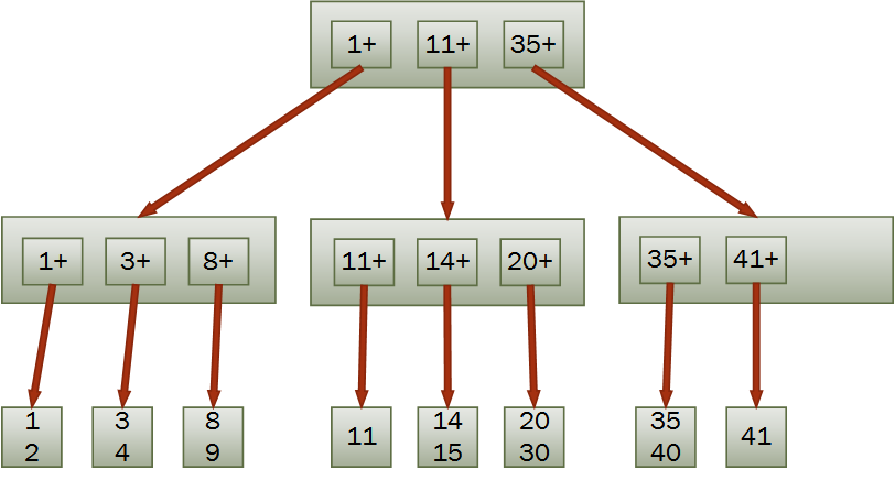
SQL Server stores a table in a tree format (a B+Tree). This is somewhat similar to a binary tree – see the Data Structures and Algorithms topic on “Searching”, and make sure you’re familiar with the concepts in there. However rather than having only two child nodes, a B+Tree parent node has many children. A B+Tree consists of two types of node:
- Leaf nodes (at the bottom of the tree) contain the actual data
- The remaining nodes contain only pointers to their child nodes
The pointers in the B+Tree are normally based on the primary key of the table – so if you know the primary key value of the row you want, you can efficiently search down the tree to find the leaf node that contains your information.
The actual row data is stored in units called “pages”. Several rows may be stored together in a page (each page is 8kB in size). A leaf node contains one page of data.
Efficient and inefficient queries
Consider our Cats table; its definition is as follows:
CREATE TABLE Cats (
  Id int IDENTITY NOT NULL PRIMARY KEY  ,
  Name nvarchar(max) NULL,
  Age int NULL,
  OwnerId int NOT NULL
)
SQL Server will store this on disk in a tree structure as described above, with the Id field as the key to that tree. So the following query will be cheap to execute – just follow down the tree to find the page containing Cat number 4:
SELECT * FROM Cats WHERE Id = 4
However the following query will be slow – SQL Server will need to find every page that contains data for this table, load it into memory if it’s not there already, and check the Age column:
SELECT * FROM Cats WHERE Age = 3
- The first query uses a “Seek”. That means it’s looking up a specific value in the tree, which is efficient
- The second query uses a “Scan”. That means it has to find all the leaf nodes of the tree and search through all of them, which can be slow
The majority of SQL performance investigations boil down to working out why you have a query containing the second example, and not of the first.
Indexes
The key tool in your performance arsenal is the ability to create additional indexes for a table, with different keys.
In a database context, the plural of index is typically indexes. In a mathematical context you will usually use indices.
Let’s create an index on the age column:
CREATE INDEX cats_age ON cats (age)
Behind the scenes SQL Server sets up a new tree (if you now have millions of cats, this could take a while – be patient!). This time the branches are labelled with age, not ID. The leaves of this tree do not contain all the cat data though – they just contain the primary key values (cat ID). If you run SELECT * FROM Cats WHERE Age = 3 and examine the execution plan, you would see two stages:
- One Seek on the new index, looking up by age
- A second Seek on the primary key, looking up by ID (this might be called a “Key Lookup”, depending on how SQL Server has decided to execute the query)
You are not limited to using a single column as the index key, here is a two column index:
CREATE INDEX cats_age_owner_id ON cats (age, owner_id)
The principle is much the same as a single-column index, and this index will allow the query to be executed very efficiently by looking up any given age + owner combination quickly.
It’s important to appreciate that the order in which the columns are defined is important. The structure used to store this index will firstly allow Microsoft SQL Server to drill down through cat ages to find age = 3. Then within those results you can further drill down to find owner_id = 5. This means that the index above is has no effect for the following query:
SELECT * FROM cats WHERE owner_id = 5
Choosing which indexes to create
Indexes are great for looking up data, and you can in principle create lots of them. However you do have to be careful:
- They take up space on disk – for a big table, the index could be pretty large too
- They need to be maintained, and hence slow down
UPDATEandINSERToperations – every time you add a row, you also need to add an entry to every index on the table
Here are some general guidelines you can apply, but remember to use common sense and prefer to test performance rather than making too many assumptions.
-
Columns that are the end of a foreign key relationship will normally benefit from an index, because you probably have a lot of
JOINs between the two tables that the index will help with. -
If you frequently do range queries on a column (for example, “find all the cats born in the last year”), an index may be particularly beneficial. This is because all the matching values will be stored adjacently in the index (perhaps even on the same page), so SQL Server can find the matching rows almost as quickly as a single-value lookup.
-
Indexes are most useful if they are reasonably specific. In other words, given one key value, you want to find only a small number of matching rows.
Agein our cat database is a very poor key, because cats will only have a small number of distinct ages.
Accessing databases through code
This topic discusses how to access and manage your database from your application level code.
The specific Database Management System (DBMS) used in examples below is Microsoft SQL Server, but most database access libraries will work with all mainstream relational databases (Oracle, MySQL, etc.). In order to provide a concrete illustration of an application layer we provide examples .NET / C# application code using the Dapper ORM (Object Relational Mapper), but the same broad principles apply to database access from other languages and frameworks (you should remember using the Entity Framework ORM in the Bookish exercise).
Direct database access
At the simplest level, you can execute SQL commands directly from your application layer like so:
using (var connection = new SqlConnection(connectionString)) {
  var command = new SqlCommand("SELECT Name FROM Owners", connection);
  connection.Open();
  var reader = command.ExecuteReader();
  while (reader.Read())
  {
    yield return reader.GetString(0);
  }
  reader.Close();
}
- A connection string, which tells the application where the database is (server, database name, and what credentials to use to log in)
- A
SqlConnection, which handles connecting to the database - A
SqlCommand, which represents the specific SQL command you want to execute - A
DataReader, which handles interpreting the results of the command and making them available to you
In this case our SQL query returns only a single column, so we just pick out the string value (the name of the Owner) from each row and return them as an enumeration.
Access via an ORM
An ORM is an Object Relational Mapper. It is a library that sits between your database and your application logic, and handles the conversion of database rows into objects in your application.
For this to work, we need to define a class in our application code to represent each table in the database that you would like to query. So we would create a Cat class with fields that match up with the columns in the cats database table. We could use direct database access as above to fetch the data, and then fill in the Cat objects ourselves, but it’s easier to use an ORM.
public class Cat
{
  [Key]
  public int Id { get; set; }
  public string Name { get; set; }
  public int? Age { get; set; }
  public DateTime? DateOfBirth { get; set; }
  [Write(false)]
  public Owner Owner { get; set; }
}

public class Owner
{
  public int Id { get; set; }
  public string Name { get; set; }
}
This example uses the Dapper ORM, which is very lightweight and provides a good illustration.
public IEnumerable<Location> GetAllLocations()
{
  using (var connection = new SqlConnection(connectionString))
  {
    return connection.Query<Location>("SELECT * FROM Locations");
  }
}
This still has a SQL query to fetch the locations, but “by magic” it returns an enumeration of Location objects – no need to manually loop through the results of the SQL query or create our own objects. Behind the scenes, Dapper is looking at the column names returned by the SQL query and matching them up to the field names on the Location class. Using an ORM in this way greatly simplifies your database access layer.
Using an ORM also often provides a slightly cleaner way of building the connection string for accessing the database, avoiding the need to remember all the correct syntax.
Building object hierarchies
In the database, each Cat has an Owner, so the Cat class defined above has an instance of an Owner. Consider the Cat and Owner classes (ignore the Key and Write attributes for now – they’re not used in this section), and take a look at the following method.
public IEnumerable<Cat> GetAllCats()
{
  using (var connection = new SqlConnection(connectionString))
  {
    return connection.Query<Cat, Owner>("SELECT * FROM Cats JOIN Owners ON Cats.OwnerId = Owners.Id");
  }
}
The method returns a list of Cats, and again Dapper is able to deduce that the various Owner-related columns in our SQL query should be mapped onto fields of an associated Owner object.
One caveat to note is that if several cats are owned by Jane, each cat has a separate instance of the owner. There are multiple Jane objects floating around in the program – the different cats don’t know they have the same owner. Depending on your application this may or may not be ok. More complex ORMs will notice that each cat’s owner is the same Jane and share a single instance between them; if you want that behaviour in Dapper, you’ll have to implement it yourself.
SQL parameterisation and injection attacks
Consider the following method, which returns a single cat.
public Cat GetCat(string id)
{
  using (var connection = new SqlConnection(connectionString))
  {
    return connection.Query<Cat, Owner>(
      "SELECT * FROM Cats JOIN Owners ON Cats.OwnerId = Owners.Id WHERE Cats.Id = @id",
      new { id }).Single();
  }
}
This uses “parameterised” SQL – a SQL statement that includes a placeholder for the cat’s ID, which is filled in by SQL Server before the query is executed.
The way we’ve written this is important. Here’s an alternative implementation:
public Cat GetCat(string id)
{
  using (var connection = new SqlConnection(connectionString))
  {
    return connection.Query<Cat, Owner>(
      "SELECT * FROM Cats JOIN Owners ON Cats.OwnerId = Owners.Id WHERE Cats.Id = " + id).Single();
  }
}
This will work. If the method were passed “1”, then the age of the cat with id 1 would be incremented.
But what if instead of “1”, a malicious user gave an input such that this method was passed the following: “1 UPDATE Cats SET Age = 2 WHERE Id = 3” (no quotation marks)? Well, the edit would go through as expected, but the extra SQL the malicious user typed in was also executed. Your attention is called to this famous xkcd comic:
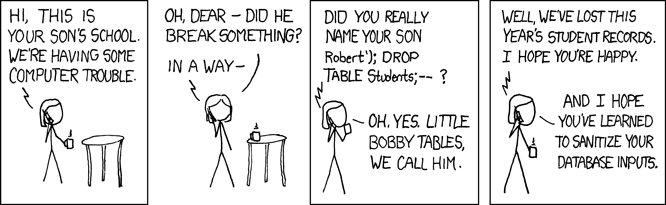
Never create your own SQL commands by concatenating strings together. Always use the parameterisation options provided by your database access library. With the first version of the GetCat method this kind of attack will not work.
Leaning more heavily on the ORM
Thus far we’ve been writing SQL commands, and asking the ORM to convert the results into objects. But most ORMs will let you go further than this, and write most of the SQL for you. An illustration of this is below.
public Cat GetCatWithoutWritingSql(int id)
{
  using (var connection = new SqlConnection(connectionString))
  {
    return connection.Get<Cat>(id);
  }
}
How does Dapper perform this magic? It’s actually pretty straightforward. The class Cat presumably relates to a table named either Cat or Cats – it’s easy to check which exists. If you were fetching all cats then it’s trivial to construct the appropriate SQL query: SELECT * FROM Cats. And we already know that once it’s got the query, Dapper can convert the results into Cat objects.
Being able to select a single cat is harder – Dapper’s not quite smart enough to know which is your primary key field. (Although it could work this out, by looking at the database). So we’ve told it – check that Cat class, and see that it’s got a [Key] attribute on the Id property. That’s enough to tell Dapper that this is the primary key, and hence it can add WHERE Id = ... to the query it’s using.
Sadly Dapper also isn’t quite smart enough to populate the Owner property automatically via this approach, and it will remain null. In this instance we don’t need it, so we take no further action, but in general you have two choices in this situation:
- Fill in the Owner property yourself, via a further query.
- Leave it null for now, but retrieve it automatically later if you need it. This is called “lazy loading”.
Lazy Loading
It’s worth a quick aside on the pros and cons of lazy loading.
In general, you may not want to load all your data from the database up-front. If it is uncertain whether you’ll need some deeply nested property (such as Cat.Owner in this example), it’s perhaps a bit wasteful to do the extra database querying needed to fill it in. Database queries can be expensive. So even if you have the option to fully populate your database model classes up-front (“eager loading”), you might not want to.
However, there’s a disadvantage to lazy loading too, which is that you have much less control over when it happens – you need to wire up your code to automatically pull the data from the database when you need it, but that means the database access will happen at some arbitrary point in the future. You have a lot of new error cases to worry about – what happens if you’re half way through displaying a web page when you try lazily loading the data, and the database has now gone down? That’s an error scenario you wouldn’t have expected to hit. You might also end up with a lot of separate database calls, which is also a bad thing in general – it’s better to reduce the number of separate round trips to the database if possible.
So – a trade off. For simple applications it shouldn’t matter which route you use, so just pick the one that fits most naturally with your ORM (often eager loading will be simpler, although frameworks like Ruby on Rails automatically use lazy loading by default). But keep an eye out for performance problems or application complexity so you can evolve your approach over time.
Migrations
Once you’re up and running with your database, you will inevitably need to make changes to it. This is true both during initial development of an application, and later on when the system is live and needs bug fixes or enhancements. You can just edit the tables directly in the database – adding a table, removing a column, etc. – but this approach doesn’t work well if you’re trying to share code between multiple developers, or make changes that you can apply consistently to different machines (say, the test database vs the live database).
A solution to this issue is migrations. The concept is that you define your database changes as a series of scripts, which are run on any copy of the database in sequence to apply your desired changes. A migration is simply an SQL file that defines a change to your database. For example, your initial migration may define a few tables and the relationships between them, the next migration may then populate these tables with sample data.
Entity Framework is one commonly-used migration framework for .NET projects, you should remember using in the Bookish Exercise
Non-relational databases
Non-relational is a catch all term for any database aside from the the relational, SQL-based databases which you’ve been studying so far. This means they usually lack one or more of the usual features of a SQL database:
- Data might not be stored in tables
- There might be no fixed schema
- Different pieces of data might not have relations between them, or the relations might work differently (in particular, no equivalent for
JOIN).
For this reason, there are lots of different types of non-relational database, and some pros and cons of each are listed below. In general you might consider using a non-relational when you you don’t need the rigid structure of a non-relational database.
Think very carefully before deciding to use a non-relational database. They are often newer and less well understood than SQL, and it may be very difficult to change later on. It’s also worth noting that some non-relational database solutions do not provide ACID transactions, so are not suitable for applications with particularly stringent data reliabilty and integrity requirements.
You might also hear the term NoSQL to refer to these types of databases. NoSQL databases are, in fact, a subset of non-relational databases – some non-relational databases use SQL – but the terms are often used interchangeably.
Key Value Stores
In another topic you’ll look at the dictionary data structure, wherein key data is mapped to corresponding value data. The three main operations on a dictionary are:
get– retrieve a value givens its key.put– add a key and value to the dictionary.remove– remove a value given its key.
A key value store exposes this exact same API. In a key value store, as in a dictionary, retrieving an object using its key is very fast, but it is not possible to retrieve data in any other way (other than reading every single document in the store).
Unlike relational databases, key-value stores are schema-less. This means that the data-types are not specified in advance (by a schema).
This means you can often store binary data like images alongside JSON information without worrying about it beforehand. While this might seem powerful it can also be dangerous – you can no longer rely on the database to guarantee the type of data which may be returned, instead you must keep track of it for yourself in your application.
The most common use of a key value store is a cache, this is a component which stores frequently or recently accessed data so that it can be served more quickly to future users. Two common caches are Redis and Memcached – at the heart of both are key value stores kept entirely in memory for fast access.
Document Stores
Document stores require that the objects are all encoded in the same way. For example, a document store might require that the documents are JSON documents, or are XML documents.
As in a key value store, each document has a unique key which is used to retrieve the document from the store. For example, a document representing a blog post in the popular MongoDB database might look like:
{
  "_id": "5aeb183b6ab5a63838b95a13",
  "name": "Mr Burns",
  "email": "c.m.burns@springfieldnuclear.org",
  "content": "Who is that man?",
  "comments": [
    {
      "name": "Smithers",
      "email": "w.j.smithers@springfieldnuclear.org",
      "content": "That's Homer Simpson, sir, one of your drones from sector 7G."
    },
    {
     "name": "Mr Burns",
     "email": "c.m.burns@springfieldnuclear.org",
     "content": "Simpson, eh?"
    }
  ]
}
In MongoDB, the _id field is the key which this document is stored under.
Indexes in non-relational databases
Storing all documents with the same encoding allows documents stores to support indices. These work in a similar way to relational databases, and come with similar trade-offs.
For example, in the blog post database you could add an index to allow you to look up documents by their email address and this would be implemented as a separate lookup table from email addresses to keys. Adding this index would make it possible to look up data via the email address very quickly, but the index needs to be kept in sync – which costs time when inserting or updating elements.
Storing relational data
The ability to do joins between tables efficiently is a great strength of relational databases such as Microsoft SQL Server and is something for which there is no parallel in a non-relational database. The ability to nest data mitigates this somewhat but can produce its own set of problems.
Consider the blog post above. Due to the nested comments, this would need multiple tables to represent in a Microsoft SQL Server databases – at least one for posts and one for comments, and probably one for users as well. To retrieve the comments shown above two tables would need to be joined together.
SELECT Users.Name, Users.Email, Comments.Content
  FROM Comments
  JOIN Users on Users.Id = Comments.Author
  WHERE Comments.Post = 1;
So at first sight, the document store database comes out on top as the same data can be retrieved in a single query without a join.
collection.findAll({_id: new ObjectId("5aeb183b6ab5a63838b95a13")})["comments"];
But what if you need to update Mr Burns’ email address? In the relational database this is an UPDATE operation on a single row but in the document store you may need to update hundreds of documents looking for each place that Mr Burns has posted, or left a comment! You might decide to store the users email addresses in a separate document store to mitigate this, but document stores do not support joins so now you need two queries to retrieve the data which previously only needed a single query.
Roughly speaking, document stores are good for data where:
- Every document is roughly similar but with small changes, making adding a schema difficult.
- There are very few relationships between other elements.
Sharding
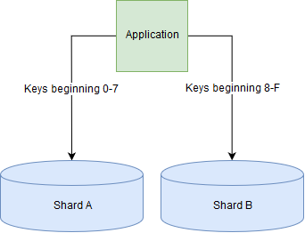
Sharding is a method for distributing data across multiple machines, it’s used when a single database server is unable to cope with the required load or storage requirements. The data is split up into ‘shards’ which are distributed across several different database servers. This is an example of horizontal scaling.
In the blog post database, we might shard the database across two machines by storing blog posts whose keys begin with 0-7 on one machine and those whose keys begin 8-F on another machine.
Sharding relational databases is very difficult, as it becomes very slow to join tables when the data being joined lives on more than one shard. Conversely, many document stores support sharding out of the box.
More non-relational databases
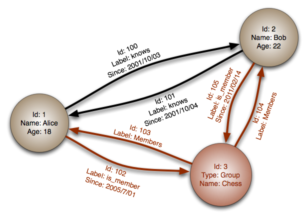
Graph databases are designed for data whose relationships fit into a graph, where graph is used in the mathematical sense as a collection of nodes connected by edges. For example a graph database could be well suited for a social network where the nodes are users and friend ships between users are modelled by edges in the graph. Neo4J is a popular graph database.
A distributed database is a database which can service requests from more than one machine, often a cluster of machines on a network.
A sharded database as described above is one type of this, where the data is split across multiple machines. Alternatively you might choose to replicate the same data across multiple machines to provide fault tolerance (if one machine goes offline, then not all the data is lost). Some distributed databases also offer guarantees about what happens if half of your database machines are unable to talk to the other half – called a network partition – and will allow some of both halves to continue to serve requests. With these types of databases, there are always trade-offs between performance (how quickly your database can respond to a request), consistency (will the database ever return “incorrect” data), and availability (will the database continue to serve requests even if some nodes are unavailable). There are numerous examples such as Cassandra and HBase, and sharded document stores including MongoDB can be used as distributed databases as well.
Further reading on non-relational databases
For practical further reading, there is a basic tutorial on how to use MongoDB from a NodeJS application on the W3Schools website.